Summary of Physical Computing and DC Motor Control
Managing a DC motor with an Arduino is shown via electromechanical relay switching and transistor-based solid-state control, including speed regulation using a potentiometer and a CdS photocell. The chapter explains transistor relay driver biasing, flyback diode protection, active-high/active-low inputs, PWM speed control using Arduino, hardware assembly on a breadboard, testing with DMM/oscilloscope, and suggestions for further modifications and experiments.
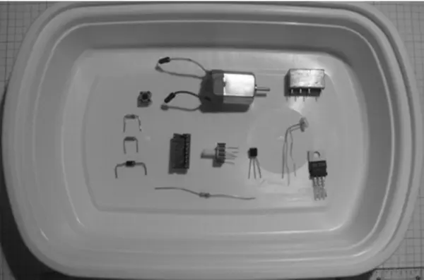
Parts used in the DC Motor Control Project:
- Arduino Duemilanove or equivalent
- TIP31C NPN Power Transistor or TIP120 NPN Darlington Transistor
- 2N2222 NPN Transistor
- 10K trimmer potentiometer
- Two 10K resistors
- 1K resistor
- CdS photocell
- Tactile push-button switch
- 1N4001 diode (flyback diode)
- 3VDC or 6VDC motor
- 16-pin IC socket
- +5VDC electromechanical relay
- Small solderless breadboard
- 22 AWG solid wires
- Digital multimeter
- Oscilloscope (optional)
- Electronic tools
Managing a DC motor through an Arduino is a straightforward task. Beyond employing a basic electric switch, there are diverse approaches to engage with a motor. Moreover, the conventional electromechanical relay can be readily substituted with a carefully chosen transistor, enabling software-based speed control. This chapter will investigate multiple strategies for DC motor control, encompassing both the conventional method of electromechanical switching via a relay and the contemporary solid-state control utilizing a transistor. Additionally, we will explore the conventional technique of speed adjustment through a potentiometer and delve into the functionality of a force-sensitive resistor. Both the potentiometer and the photocell qualify as input devices for physical computing, thus meriting a comprehensive discussion within this chapter. By integrating the previously discussed electronic principles from earlier units with the forthcoming topics, I will elucidate both electronic prototyping and software development’s supplementary remix techniques within this Project.
Arduino Duemilanove or equivalent
TIP31C NPN Power Transistor or TIP120 NPN Darlington Transistor
2N2222 NPN Transistor
10K trimmer potentiometer
2 10K resistors
1K resistor
CdS photocell
Tactile push-button switch
1N4001 diode
3VDC or 6VDC motor
16-pin IC socket
+5VDC electromechanical relay
Small solderless breadboard
22 AWG solid wires
Digital multimeter
Oscilloscope (optional)
Electronic tools
How It Works
Prior to the adoption of transistors as direct drivers for electronic circuits, electromechanical relays served as the mechanism to regulate high-current electrical loads. Commencing the discourse on physical-computing DC motor control, I will initiate with a practical investigation of a transistor relay driver circuit. Figure 4-4 illustrates a schematic block diagram of a fundamental transistor relay driver circuit.
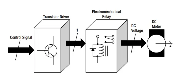
Figure 3 displays a circuit schematic outlining the standard configuration of a transistor relay driver block diagram.
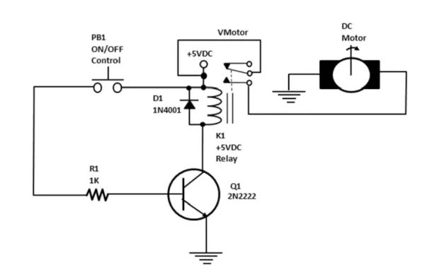
A Base Biasing Transistor Driver Circuit
Depressing switch PB1 initiates the flow of current via resistor R1, thereby facilitating biasing of the transistor. This approach to managing current through the transistor is recognized as base biasing. The simplicity of this biasing method arises from the presence of a sole resistor linked in series with a +5VDC power source and the transistor’s base circuit. The current coursing through the resistor proves ample for either activating the NPN transistor or placing it in a state of saturation mode. To compute the biasing or base current within the transistor driver circuit, one may employ the subsequent analytical equation:
Ib= (Vcc- Vbe )/Rb
where
- IB is the base current.
- VCC is the collector supply voltage.
- VBE is the base-emitter junction voltage.
- RB is the base resistor (R1is equal to RB in this design).
Utilizing Figure 3 in conjunction with the equation provided earlier, you have the means to ascertain IB. The subsequent activity illustrates the sequential procedures essential for accomplishing this task:
1. First, write down the original analysis equation:
Ib= (Vcc-Vbe)/ Rb
2. Next, substitute circuit parameter values into the analysis equation:
Ib= (5VDC- 0.7V )/1K
3. Finally, solve for IB:
Ib= 4.3VDC/1K
Ib= 0.0043A or 4 .3mA
By utilizing the Multisim circuit simulation software, you can effortlessly construct a virtual transistor circuit. When the electrical switch is in the open position, the base current remains exceedingly minute (on the order of picoamperes [pA]), leading to the electromechanical relay remaining unpowered, as portrayed in Figure 4(a). The 69.8Ω resistor symbolizes the resistance of the electromechanical relay coil as it would be measured using an ohmmeter. Upon closing the electrical switch, biasing of the transistor takes place, thereby energizing the electromechanical relay. This scenario of transistor base biasing is illustrated in Figure 4(b).
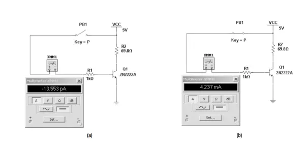
Operating in saturation mode, the NPN transistor establishes a pathway for the current originating from the +5VDC power source. This current flows through both the electromechanical relay’s coil and the collector-emitter junctions of the NPN transistor (2N2222), eventually grounding itself. As the current courses through the coil of the electromechanical relay, it transitions into a conductive state referred to as energization. The flow of current within the coil windings generates a magnetic field, thereby inducing the coil to attract its moveable contact, known as the armature. This attraction is heightened through the use of a robust iron core within the relay, intensifying the connection between the coil and the armature. The armature, responding to the magnetic field, establishes contact with the normally open (NO) contact of the electromechanical relay. Consequently, the Vmotor power supply (+5VDC) is effectively routed into the external control circuit, permitting the current to course through the DC motor and thereby activating it.
Releasing switch PB1 results in an open circuit at the base, effectively removing the current bias applied to the NPN transistor. As the current supply to the coil is interrupted, the electromechanical relay’s contacts disengage, leading to their de-energization. The magnetic field, previously generated during the energization process, dissipates, allowing the armature to revert to its normally closed (NC) position contact. Consequently, the external control circuit disengages, halting the rotation of the DC motor. It’s worth noting that the electromechanical relay’s contacts possess an ampacity rating, enabling them to manage high-current components such as incandescent bulbs and low-power motors. These contacts can have ampacity ratings ranging from as low as 1A to as high as 10A. This characteristic empowers the Arduino to readily execute industrial control applications on a workbench setting.
D1: Flyback Diode
The electromechanical relay coil essentially functions as an inductor with the capacity to retain electric current within its winding structure. Upon energization and subsequent de-energization of the coil, the inductor experiences charging and discharging processes accordingly. Upon de-energization of the electromechanical relay coil, the accumulated energy (electric current) necessitates release or discharge through a designated grounding pathway. In the context of a relay driver circuit, this grounding route is facilitated by the transistor. The stored electric current within the relay coil attains its maximum amplitude (IP [peak current]) and can pose significant risk to delicate electronic components during the discharge process, potentially leading to severe damage when energy is dissipated into a grounding medium.
The transistor functions as a conduit for grounding the electromechanical relay, making it susceptible to potential damage from the maximum IP value. The inclusion of a diode across the coil serves to channel this electrical energy back through the relay windings using a flyback technique for suppressing electric current. This flyback approach enables the diode to absorb the peak current generated by the inductor during the charging phase and that of the coil when the electromechanical relay is de-energized. As the transistor transitions to the off state, particularly during the de-energization process of the electromechanical relay, the diode becomes forward biased. This bias redirects the peak current away from the transistor, enabling it to travel through the coil of the electromechanical switch.
A flyback diode is alternatively referred to as a snubber, freewheeling, suppressor, or catch diode. Illustrated in Figure 5 is the Multisim circuit representation of an electromechanical relay coil paired with a parallel-connected flyback diode. In Figure 5(a), the relay undergoes energization, signifying the charging of the inductor. Conversely, Figure 5(b) portrays the de-energized state of the relay, indicative of the inductor’s discharge. Notably, the peak current during discharge is considerably more substantial in terms of magnitude and electrical units (measured in milliamperes) when compared to the coil’s energization phase (measured in nanoamperes).
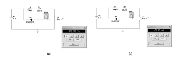
Figure 5 depicts Multisim circuit models for transistor drivers: (a) inductor charging (relay coil energized), and (b) inductor discharging (relay coil de-energized). The diagrams show an unbiased transistor in (a) and a base-biased operation in (b).
Experimenting with a Transistor Relay Driver DC Motor Control Circuit
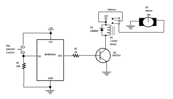
Constructing a DC motor control circuit using a transistor relay driver in conjunction with an Arduino is a straightforward task. The Arduino assumes the role of an intelligent processing interface, receiving control signals from tactile push-button switches and issuing commands to activate the transistor relay driver, thereby governing the DC motor’s operation. The circuit schematic diagram for this uncomplicated DC motor control setup is illustrated in Figure 6.The button sketch employed in the bird project is transferred to the Arduino, enabling the activation of the DC motor through the transistor relay driver circuit.
Let’s delve deeper into the physical-computing aspects of the DC motor control circuit. The resistor in tandem with the tactile push-button switch functions as an input transducer or sensor. This is due to the conversion process that occurs, translating mechanical action (pressing the switch’s internal contacts using a mini-plunger-spring mechanism) into the generation of a digital-level electrical control signal (either +5VDC or a binary 1 logic level). Once the tactile switch button is released, the mini-plunger-spring mechanism prompts it to return to its original position, causing the binary 1 logic level control signal to transition into a 0 logic level signal.
The configuration where the tactile push-button switch is positioned before the 10K resistor is recognized as an active-high digital input circuit. If an inverse or contrary transducer operation is necessary, rearranging the positions of the push-button switch and the 10K resistor accomplishes this specification. This reversed electrical control signal function is referred to as an active-low digital input circuit.
Figure 7 illustrates the analysis of the Multisim circuit model, presenting the outcome in the form of output voltage readings showcased on a digital voltmeter. Meanwhile, Figure 8 showcases a physical-computing DC motor control system based on Arduino, featuring an active-low digital input circuit. For contrast, an active-high digital input circuit for the Arduino-based physical-computing DC control is displayed in Figure 9.
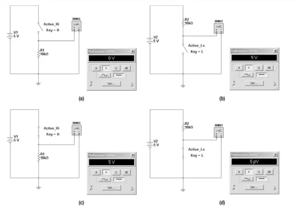
Figure 7. presents the voltage of an active-high digital input circuit with the switch in an open state, along with the voltage of an active-low digital input circuit with the switch also open (b). Notably, the measured voltages exhibit an inversion between the active-high and active-low digital input circuit configurations.
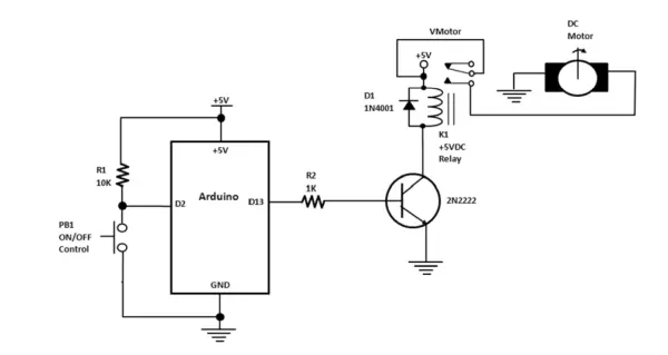
Figure 8. showcases the schematic diagram of a physical-computing DC motor control system utilizing an active-low configuration.
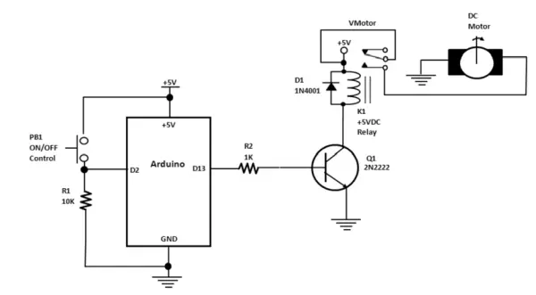
Figure 9 displays the schematic diagram of a physical-computing DC motor control system employing an active-high configuration.
Electromechanical Relay Preparation
During the phase of prototyping fundamental physical-computing DC motor control circuits on a solderless breadboard, you have the option to enhance the connection quality of the +5VDC electromechanical relay pins with the internal spring terminals. A viable strategy involves placing the electromechanical relay within an IC socket, which enhances the contact force of the electrical pins and eliminates the potential for intermittent circuit connections during the project assembly. This approach is depicted in Figure 11.
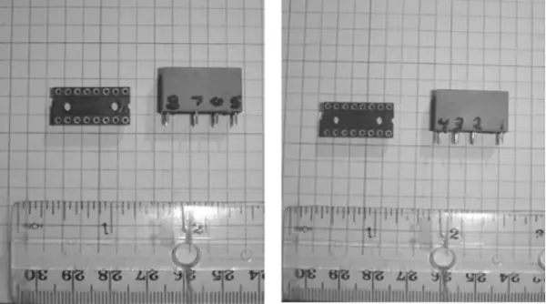
Figure 10 showcases the pinout information clearly labeled on both faces of the electromechanical relay.
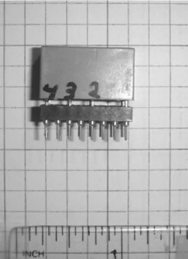
Figure 11 depicts the utilization of an IC socket to enhance the ease of inserting the electromechanical relay onto the solderless breadboard.
As the project involves only a small number of components, you have the flexibility to position them in close proximity, as demonstrated in Figure 12. Employing stranded core wire along with preformed jumper wires facilitates the organization of circuit connections on both the breadboard and the Arduino. The Arduino board itself serves as the source of +5VDC supply, powering both the control circuit and the DC motor.
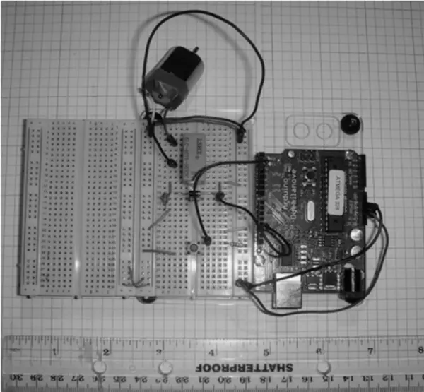
Figure 11 displays the implementation of an IC socket for the purpose of enhancing.
The setup depicted in Figure12 is configured as an active-high digital input circuit. Upon pressing and holding the tactile push-button switch, the Arduino generates an output control signal (approximately +5VDC). This signal biases the 2N2222 NPN transistor, initiating the activation of the electromechanical relay. Consequently, the contacts of the electromechanical relay transition from the normally closed (NC) position to the normally open (NO) position, enabling the +5VDC power supply to engage the DC motor. Releasing the button discontinues the biasing current within the transistor relay driver circuit, leading to the interruption of the +5VDC power source from the DC motor and thus halting its rotation.
The Basics of Physical Computing with Electric Motors
The initial pages of this chapter elucidated the notion of controlling a DC motor through the integration of a transducer (or sensor), microcontroller, and transistor relay driver, demonstrated through simulated circuits and an actual control project. Utilizing an electromechanical relay aligns with the conventional method for propelling electric motors, primarily due to the relay’s switching contacts capable of managing substantial currents, often measuring in amperes. Electric motors fundamentally function as electromechanical devices, as they convert electrical signals (comprising voltage and/or current) into mechanical motion. To surmount the challenges inherent in rotation mechanics, a considerable inrush current must be sourced from the power supply responsible for propelling the electromechanical component.
In the instance of the discussed straightforward physical-computing DC motor control project, the electromechanical relay shouldered the responsibility of supplying power by means of a set of contacts with a high ampacity rating. However, an alternate method exists for motor control: substituting the electromechanical relay with a power transistor. Electric motors hinge on two pivotal parameters – torque and speed – necessitating an adept means of control for these factors. Here, a microcontroller combined with a power transistor emerges as a proficient and streamlined strategy, ensuring consistent and precise regulation of torque and speed for electric motors.
Embedded within the Arduino is a specialized computational and mathematical approach that employs a well-established procedure (algorithm) to ensure precise control of torque and speed for electric motors. An algorithm represents a systematic series of steps for performing calculations. The microcontroller constantly supervises the output of the electric motor, employing feedback from a transducer or sensor that yields voltage or current signal data associated with the motor’s torque and/or speed. The microcontroller’s embedded software perpetually monitors these signal data for any deviations and, if such deviations arise, it implements adjustments to the output signal responsible for controlling the driving circuit. Hence, the transducer or sensor, entrusted with monitoring the motor’s output parameters, indirectly contributes to the physical-computing activity exerted upon the electric motor. This relationship is illustrated in Figure 13, portraying a standard system block diagram for a DC motor controller founded on physical computing principles.
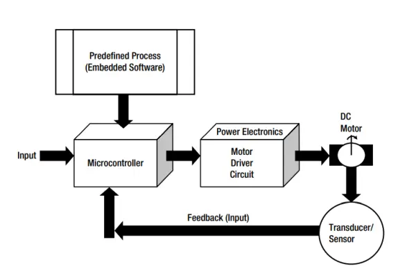
Figure 13 illustrates the system block diagram delineating the control of the DC motor.
Achieving Motor Speed Control with Physical Computing
Up until this point in the chapter, the focus has been primarily on the fundamental control of DC motors, essentially involving their activation and deactivation. The subsequent sections of this chapter will delve into the realm of regulating the motor’s speed through the application of physical-computing methods. You will engage with input sensor circuits, specifically employing a potentiometer and a photocell, to facilitate interaction with the DC motor and attain speed control.
Potentiometer Input Control
By toggling the base at a predefined frequency, the transistor is enabled to deliver an averaged current to the stator of the DC motor, effectively regulating the speed of the electromechanical unit. Illustrated in Figure 14 is a common approach to controlling DC motor speed, utilizing the Arduino as the generator of the PWM signal.
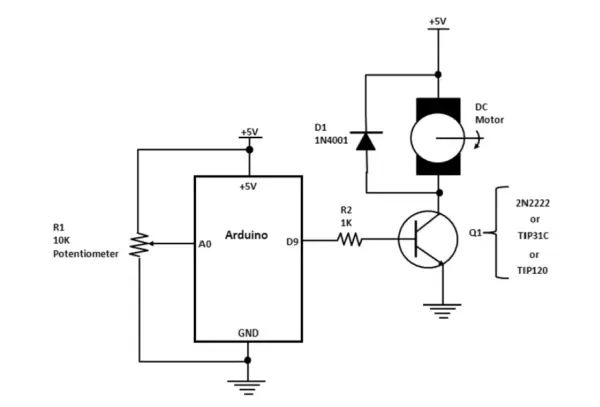
Figure 14 displays the schematic diagram of a physical-computing DC motor speed controller.
The assembly of the circuit on the solderless breadboard involves a minimal number of components and wiring. Additionally, just two jumper wires are required to connect the potentiometer and the base of the 2N2222 transistor to the Arduino’s single inline header connectors. The conclusive motor speed controller prototype is depicted in Figure 15.
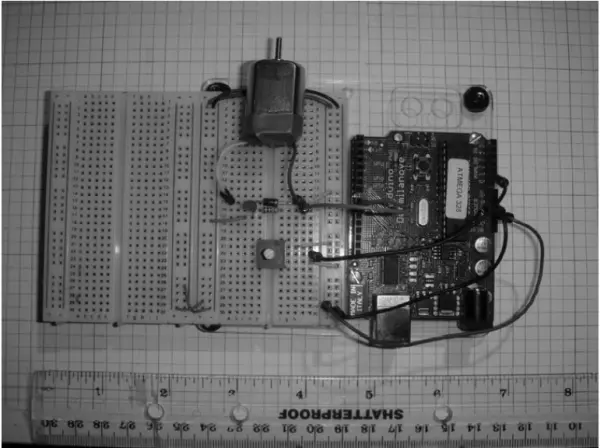
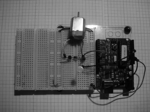
Figure 15 illustrates a DC motor speed controller based on physical computing, assembled using a solderless breadboard.
As previously explained, motor speed control is achieved using the 10KΩ potentiometer. Tweaking this component enables the ATmega328 microcontroller of the Arduino to generate a seamless sequence of pulses. These pulses serve to bias the 2N2222 transistor effectively, allowing it to efficiently drive the small DC motor. To observe the PWM signal, connecting an oscilloscope involves attaching one test lead to the base of the transistor driver and the other lead to a ground point. Figure 16 demonstrates the configuration for attaching an oscilloscope to the base lead of the 2N2222 NPN transistor. The practical arrangement for these measurements is presented in Figure 17.
Rotating the shaft of the potentiometer induces a corresponding alteration in the duty cycle value, which varies proportionally with the degree of resistance. As the resistance of the potentiometer increases, the duty cycle value expands. With a resistance set to its maximum value (10KΩ), the duty cycle attains 100 percent, causing the small DC motor to operate at its full-rated speed.
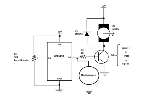
- Figure 16 illustrates the circuit schematic diagram depicting the Arduino-controlled DC motor setup, complete with an oscilloscope for observing the PWM signals.
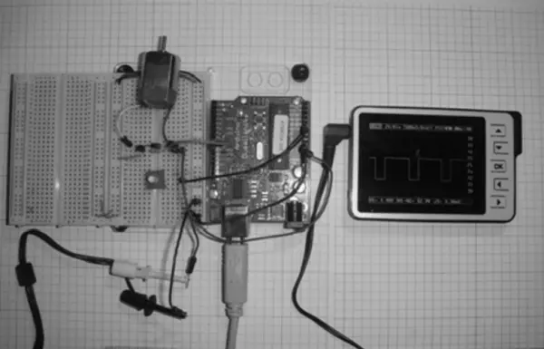
- Figure 17 displays the circuit schematic diagram outlining the procedure for connecting an oscilloscope to visualize the PWM signals generated by the Arduino.
- Figure 18 provides a detailed view of the PWM control signal generated by the Arduino, revealing a sequence of well-defined square-wave pulses.
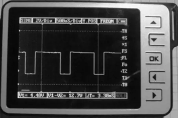
- Figure 18 illustrates the PWM control signal generated by the Arduino to regulate motor speed.
The 2N2222 Transistor Pinout
It’s crucial to emphasize that not all NPN transistors share identical characteristics. The pinout arrangement of the 2N3904 NPN transistor places the emitter on the left side of the three-pin component. The base occupies the central lead, while the collector resides on the immediate right. Conversely, for the 2N2222 transistor, the emitter is situated on the right side, and the collector is positioned on the left side.
Figure 17 outlines the pinout configuration for the 2N2222 transistor, ensuring the accurate operational functionality of both the speed control circuit and the basic motor control project.
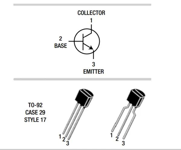
Figure 19 presents the pinout diagram for the 2N2222 NPN transistor (adapted from ON Semiconductor datasheet).
The Motor Speed Control Software
Having assembled the electronic hardware, the next step involves implementing the sketch to finalize the project construction. This sketch empowers the Arduino to interpret the analog position of the potentiometer and subsequently generate a PWM signal correlated to the angular positioning of the wiper arm. The sketch is thoughtfully annotated, thereby simplifying potential adjustments to the analog or digital port pins. The motor speed control sketch is depicted in Listing 1 for reference.
Listing 1. The Motor Speed Control Sketch
int motorPin = 9; // motor connected to digital pin 9
int analogPin = 0; // potentiometer connected to analog pin 0
int val = 0; // variable to store the read value
void setup()
{
pinMode(motorPin, OUTPUT); // sets the pin as output
}
void loop()
{
val = analogRead(analogPin); // read the input pin
analogWrite(motorPin, val / 4); // analogRead values go from 0 to 1023,
analogWrite ➥
values from 0 to 255
}
A concluding point concerning the functioning of the physical computing-based controller: upon uploading the motor speed control sketch to the Arduino, the behavior of the electromechanical component may initiate at a low, medium, or high speed, contingent upon the positioning of the 10KΩ potentiometer.
Light Detection Input Control
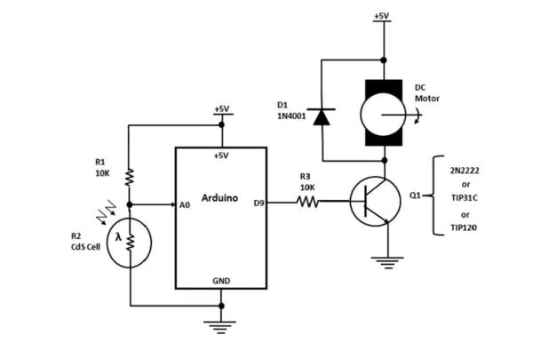
In the concluding phase of the project that delves into human interaction and control within the physical realm, we will fine-tune the speed of the DC motor utilizing light. By establishing a proportional voltage grounded in the resistance of the CdS photocell, the appropriate duty cycle for the PWM output control signal is achieved through the Arduino computing platform. When ambient light is present, positioning an object (such as a hand) over the CdS photocell will amplify the DC motor’s speed. In scenarios where the light sensor detects the absence of an object, the DC motor will rotate at a moderate pace. Conversely, if a light source illuminates the sensor, the DC motor will come to a complete stop. Figure 20 outlines the circuit schematic diagram for the light-activated DC motor speed controller.
The motor speed control sketch maintains its structure, except for the substitution of the 10KΩ potentiometer with the light detection circuit portrayed in the circuit schematic diagram illustrated in Figure 20. The ultimate project assembly is presented in Figure 21. The strategic arrangement and orientation of the CdS photocell yield optimal results, facilitated by the swift responsiveness of the Arduino computing platform in adapting the DC motor’s speed in accordance with fluctuating light levels. The transition in motor speed, characterized by a gradual acceleration and deceleration based on shifts in ambient lighting, unfolds smoothly with minimal or negligible instances of acceleration adjustment hesitation.
Final Testing of the Devices
Within this chapter, a sequence of testing procedures was outlined to identify potential flaws during the construction of hardware circuits. Employing tools like a Digital Multimeter (DMM) and an oscilloscope, these testing methodologies can be verified on the workbench. It’s important to note that the results might exhibit a variance of up to +/-10 percent contingent on the specific manufacturer of the testing instruments. During the testing process, ensure the correctness of the wiring before applying voltage to the Arduino and the accompanying circuits. The “How it Works” segment within this chapter serves as a valuable resource to confirm the accurate functionality of the circuit on the breadboard. Additionally, scrutinize the sketch within the Arduino IDE editor for any typographical errors that could lead to improper operation of the hardware device.
Further Discovery Methods
Numerous avenues for exploration are available within the context of the two projects featured in this chapter. One such avenue involves altering the operational dynamics of the basic DC motor control facilitated by a transistor relay driver circuit. Rather than employing an active-high switch for control, consider employing an active-low digital input configuration. Figure 8, as presented earlier in the chapter, serves as a guide for the configuration’s wiring arrangement during this exploration.
For the second task, consider rearranging the placement of the 10K resistor and the CdS photocell to enable the motor speed to escalate in response to ambient (usual) light conditions, illustrated in Figure 4-21. Moreover, substitute the 2N2222 transistor with either a TIP31C or TIP120 transistor. Incorporate a DC motor with a higher operational current and voltage rating and take note of the ensuing speed control dynamics. As you undertake these modifications, it’s advisable to comprehensively document the design process within a lab notebook. Record the adjustments made to the sketch for the novel DC motor speed controller that you’ve devised.
- How does the transistor relay driver biasing work?
Depressing the push-button passes current through the base resistor to the transistor base, producing base current IB = (Vcc - Vbe)/Rb which biases the transistor into saturation to drive the relay coil. - Can I replace the electromechanical relay with a transistor?
Yes, the chapter explains substituting the electromechanical relay with a power transistor like TIP31C or TIP120 for solid-state motor control. - What is the purpose of the flyback diode?
The flyback diode across the relay coil redirects the inductor's discharge current when de-energized, protecting the transistor from damaging peak currents. - How is motor speed controlled with a potentiometer?
The Arduino reads the 10K potentiometer analog value and outputs a PWM signal whose duty cycle (via analogWrite) biases the transistor to vary motor speed. - Does the CdS photocell work for speed control?
Yes, replacing the potentiometer with the CdS photocell lets ambient light change the analog input so the Arduino adjusts PWM duty cycle and motor speed accordingly. - How are active-high and active-low input circuits configured?
Active-high places the tactile switch before the pull-down resistor so pressing yields +5V; swapping the switch and 10K resistor yields an active-low configuration. - What testing tools are recommended?
Use a digital multimeter and optionally an oscilloscope to verify voltages and observe the PWM signal; results may vary by +/-10 percent by instrument. - How do I observe the PWM signal?
Connect an oscilloscope probe to the transistor base and the reference lead to ground to view the Arduino-generated square-wave PWM. - What should I check before powering the circuit?
Verify wiring correctness on the breadboard and inspect the Arduino sketch for typographical errors before applying voltage. - What further modifications are suggested?
Try active-low switching, swap the resistor and photocell to invert light response, or use TIP31C/TIP120 and a higher-current motor to explore speed control dynamics.