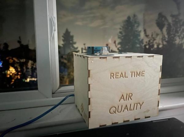
Air Quality Prediction is a project that balances Arduino development and Machine Learning. I have always found the world of machine learning captivating but was never able to run models on real-time data. Arduinos provide the solution with a vast array of sensors supported on their microcontrollers. As a result, I knew that I wanted to explore Machine Learning with Arduinos for my Side Project in Mrs. Berbawy’s Principles of Engineering Class. In this project, we will use past levels of temperature, humidity, pressure, and air quality to predict air quality in the future.
This Instructable will go in-depth on how to build a machine learning model from scratch using Python. Then, we will explore how to feed data from the Arduino to your computer and run it through a model to generate a prediction.
Supplies
Materials:
- Arduino Uno
- Adafruit BME 280 – Temperature, Humidity, and Pressure Sensor
- Grove HM3301 & Grove Cable (comes with sensor) – Laser PM2.5 Dust Sensor
- Grove Base Shield
- 4 Jumper Cables
- USB Printer Cable
- 1/8 inch wood & acrylic
- Gorilla Glue
Software:
- Python
- Arduino IDE
- Jupyter Lab / Jupyter Notebook
Python Libraries:
Step 1: Collecting Data
To train the model, we need to have data to feed it. For this project, as I mentioned earlier, I chose to train it with datasets from Napa County, California, since it is prone to wildfires, and I live nearby. However, the following methods can definitely apply to other locations of interest.
First off, we will need Air Quality Data. This will be the Y-value for our machine learning model to predict. The Environmental Protection Agency offers Air Quality Data for various detection sensors throughout the United States. Most counties have at least one sensor.
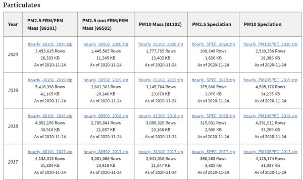
1) Scroll to the Hourly Data Section, and then scroll to the Particulates Section. There is a daily and an hourly section, so you must scroll past the daily section and to the hourly section.
2) For this project, I chose to download all data since 2017, but the reader may choose to acquire additional or fewer data. More data is always beneficial for the model, but all processes throughout this project will take slightly longer to complete as a result. I downloaded the zip files from the PM2.5 FRM/FEM Mass (88101) column for the years 2017 – 2020.
3) Using pandas, I filtered the data by location and stored the CSV into a pandas.DataFrame() object.
data_2017 = pd.read_csv(r"Data\AirQuality\EPA_AQ\Hourly\hourly_88101_2017.csv")
4) I clipped all of the values by the “County Name” column in the dataset.
df_2017 = data_2017.loc[data_2017['County Name']=='Napa']
5) I did the following for each year, concatenated the data into one DataFrame()using the following segment of code, and then saved the DataFrame() as a CSV.
df_all = pd.concat([df_2017,df_2018,df_2019,df_2020])
df_all.to_csv(r"Data\AirQuality\EPA_AQ\Hourly\full_aq.csv")
6) Lastly, I noted the latitude and longitude of my chosen point.
Next, we will need data for temperature, humidity, and pressure. These are the X-values that will be inputted into our model. Although the EPA had these files as well, it turns out that many of the counties have little to no data. The ERA-5 Climate Reanalysis Dataset provides a comprehensive set of variables across the world at hourly intervals and a decent resolution.
1) I went to the Download Data Tab & selected the following variables: 2m dewpoint temperature, 2m temperature, and surface temperature.
2) I selected every year since 2017. Then, I selected every month, day, and hour.
3) For the geographic range of data, I selected a rectangular grid of data that included my chosen point.
4) Lastly, I downloaded the data as a NetCDF.
Step 2: Preprocessing Data
After the iterative testing of multiple models and architecture adjustments, the Long Short Term Memory (LSTM) network proved to be the most effective model in this particular application. In short, the LSTM is a Recurrent Neural Network, meaning that it specializes in time series data. When humans make judgments, we have context, which allows us to remember past events and apply what we learned to the present. When we read books, we don’t start in the middle! Similarly, the LSTM has data from multiple time steps in the past to inform the current prediction. For more information, here is the documentation.
Before we start, I imported the following libraries and loaded the saved dataset.
import pandas as pd
import numpy as np
from matplotlib import pyplot as plt
import tensorflow as tf
from tensorflow.keras.models import Sequential
from tensorflow.keras.layers import Dense, Dropout, LSTM
from sklearn.metrics import mean_absolute_error
Preprocessing Data
1) First, we want to make sure every variable has no bias. To do this, we will normalize the data by ensuring that data from each variable lies between 0 and 1.
If we skipped this step, the model would have a hard time learning. Throughout the learning process, the data is multiplied by weights that are constantly tweaked to maximize the accuracy of the output. A weight applied to a variable that ranges from 0 to 1000 will be more influential than a weight applied to a variable that ranges from 1 to 10. This unstable learning phase will have larger errors and take longer to optimize. When we scale our data, this problem is eliminated and the proportions within every variable are maintained.
mns = data.min(axis=0)
data = data-data.min(axis=0)
mxs = data.max(axis=0)
data = data / data.max(axis=0)
extremes = pd.DataFrame({"min":mns, "max":mxs})
extremes.to_csv(r"..\Data\Datasets\Normalization\norm.csv")
2) Next, we must lag our data to generate the timesteps for the LSTM model. Each input in an LSTM model has the shape [T x N] where T is the number of timesteps and N is the number of variables. Having a lag of 4 timesteps was able to produce the optimal result, but the following algorithm can apply to any number of timesteps.
def lagGen(X,y,lag):
    Xs = []
    Ys = []
    for i in range(len(X)-lag):
        Xs.append(list(X[i:i+lag]))
        Ys.append(y[i+lag])
    return np.array(Xs),np.array(Ys)
3) I split the data into individual sets for training and testing. Training data will be used to train the model. The testing data will be used to assess the final and overall accuracy of the model.
X_train, X_test, y_train, y_test = train_test_split(X_lagged,y_lagged, test_size=0.1, random_state=42)
Step 3: Training the Model
The Model involves 4 layers: the input layer, the LSTM layer, the Dropout Layer, and the output Layer. The LSTM layer has 8 cells. Here, the Adam optimizer is used. We want to minimize the Mean Absolute Error (MAE), our loss function. After iterative testing, I have found that 50 epochs (the number of times the entire dataset is fed) with a batch size of 32 are enough to reach the minimum MAE.
model = Sequential()
model.add(LSTM(8, input_shape = (X_train.shape[1], X_train.shape[2])))
model.add(Dropout(rate = 0.2))
model.add(Dense(1,activation = 'relu'))
model.compile(optimizer = 'adam',loss = 'mean_absolute_error',metrics = ['mean_absolute_error','mean_squared_error','accuracy'])
out = model.fit(X_train, y_train, epochs = 50,batch_size = 32)
Model Accuracy:
We will run our model on the testing data to see how well it predicts data it has not seen before. The model achieved a MAE of 2.56 micrograms.
predictions = model.predict(X_test)
print("Testing MAE ",mean_absolute_error(y_test, predictions)*mxs["PM2.5"])
Saving the Model:
model_json = model.to_json()
with open(r"..\Models\LSTM_OneLoc_v3\LSTM.json", "w") as json_file:
    json_file.write(model_json)
model.save_weights(r"..\Models\LSTM\LSTM.h5")
Step 4: Collecting Real Time Data With the Arduino Uno
The following C++ Program was written in the Arduino IDE to collect data from the BME280 and HM3301 Sensors. This program was created by merging and truncating the example programs of each sensor. Credit for the individual programs goes to the developers of each sensor.
#include <Seeed_HM330X.h>
#include <Wire.h>
#include <SPI.h>
#include <Adafruit_Sensor.h>
#include <Adafruit_BME280.h>

#define BME_SCK 13
#define BME_MISO 12
#define BME_MOSI 11
#define BME_CS 10

#define SEALEVELPRESSURE_HPA (1013.25)

Adafruit_BME280 bme; // I2C
//Adafruit_BME280 bme(BME_CS); // hardware SPI
//Adafruit_BME280 bme(BME_CS, BME_MOSI, BME_MISO, BME_SCK); // software SPI

HM330X aq;
uint8_t buf[30];


const char* str[] = {"sensor num: ", "PM1.0 concentration(CF=1,Standard particulate matter,unit:ug/m3): ",
                     "PM2.5 concentration(CF=1,Standard particulate matter,unit:ug/m3): ",
                     "PM10 concentration(CF=1,Standard particulate matter,unit:ug/m3): ",
                     "PM1.0 concentration(Atmospheric environment,unit:ug/m3): ",
                     "PM2.5 concentration(Atmospheric environment,unit:ug/m3): ",
                     "PM10 concentration(Atmospheric environment,unit:ug/m3): ",
                    };

HM330XErrorCode print_result(const char* str, uint16_t value) {
    if (NULL == str) {
        return ERROR_PARAM;
    }
    //Serial.print(str);
    Serial.print(value);
    Serial.print(" ");
    return NO_ERROR;
}

/*parse buf with 29 uint8_t-data*/
HM330XErrorCode parse_result(uint8_t* data) {
    uint16_t value = 0;
    if (NULL == data) {
        return ERROR_PARAM;
    }
    for (int i = 1; i < 8; i++) {
        value = (uint16_t) data[i * 2] << 8 | data[i * 2 + 1];
        print_result(str[i - 1], value);

    }

    return NO_ERROR;
}

HM330XErrorCode parse_result_value(uint8_t* data) {
    if (NULL == data) {
        return ERROR_PARAM;
    }
    for (int i = 0; i < 28; i++) {
        Serial.print(data[i], HEX);
        Serial.print("  ");
        if ((0 == (i) % 5) || (0 == i)) {
            Serial.println("");
        }
    }
    uint8_t sum = 0;
    for (int i = 0; i < 28; i++) {
        sum += data[i];
    }
    if (sum != data[28]) {
        Serial.println("wrong checkSum!!!!");
    }
    Serial.println("");
    return NO_ERROR;
}

// BME280 METHODS ---------

void printValues() {
    Serial.print(bme.readTemperature());
    Serial.print(" ");
    Serial.print(bme.readPressure());
    Serial.print(" ");
    Serial.print(bme.readAltitude(SEALEVELPRESSURE_HPA));
    Serial.print(" ");
    Serial.print(bme.readHumidity());
}


/*30s*/
void setup() {
    Serial.begin(115200);
    while(!Serial);
    //Serial.println("Serial start");
    if (aq.init()) {
        Serial.println("HM330X init failed!!!");
        while (1);
    }


    unsigned status;
    status = bme.begin();
    if (!status) {
        Serial.println("Could not find a valid BME280 sensor, check wiring, address, sensor ID!");
        Serial.print("SensorID was: 0x"); Serial.println(bme.sensorID(),16);
        Serial.print("        ID of 0xFF probably means a bad address, a BMP 180 or BMP 085\n");
        Serial.print("   ID of 0x56-0x58 represents a BMP 280,\n");
        Serial.print("        ID of 0x60 represents a BME 280.\n");
        Serial.print("        ID of 0x61 represents a BME 680.\n");
        while (1) delay(10);
    }
    delay(5000);
    //Serial.println("-- Default Test --");
    //Serial.println();

}


void loop() {

    if (aq.read_sensor_value(buf, 29)) {
        Serial.println("HM330X read result failed!!!");
    }
    //parse_result_value(buf);
    parse_result(buf);
    Serial.println();
    printValues();
    Serial.println();
    delay(10000);

}
Step 5: Passing Real Time Data Into ML Model
The following program collects data from the Arduino using the Serial Port and the PySerial library. Then, it passes the data into the model, so our final prediction can be made.
Opening the Model
json_file = open('Models\LSTM\LSTM', 'r')
loaded_model_json = json_file.read()
json_file.close()
model = model_from_json(loaded_model_json)
model.load_weights("Models\LSTM\LSTM.h5")
print("Loaded model from disk")
Opening the Arduino
arduino = serial.Serial("com3",115200)
Grabbing Data from the Arduino
def grab_set():
    aq = arduino.readline()
    aq_row = str(aq[0:len(aq)].decode("utf-8"))
    air_quality = aq_row.split()[2]

    met = arduino.readline()
    met_row = str(met[0:len(met)].decode("utf-8"))
    m = met_row.split()
    temp, pressure, alt, hum = float(m[0]), float(m[1]), float(m[2]), float(m[3])
    return float(air_quality), temp, pressure/1000, hum
Creating the Prediction
cr = datetime.datetime.now().hour-1
while(1):
    hr = datetime.datetime.now().hour
    aq, temp, pressure, hum = grab_set()
    if(hr!=cr):
        cr = hr
        date = (datetime.datetime.now().month*100 + datetime.datetime.now().day+200)%1231
        print()
        print("actual: ",date,cr,hum,pressure,temp,aq)
        print()
        date = (date - norm["min"].loc[0]) / (norm["max"].loc[0])
        h = (cr - norm["min"].loc[1]) / (norm["max"].loc[1])
        hum = (hum - norm["min"].loc[2]) / (norm["max"].loc[2])
        pressure = (pressure - norm["min"].loc[3]) / (norm["max"].loc[3])
        temp = (temp - norm["min"].loc[4]) / (norm["max"].loc[4])
        aq = (aq - norm["min"].loc[5]) / (norm["max"].loc[5])

        rem = [date,h,hum,pressure,temp,aq]
        data.insert(0,rem)
        rem = []

        if(len(data)>4):
            data=data[:-1]
        if(len(data)==4):
            print("Prediction: ",model.predict(np.array([data]))*norm["max"].loc[5]-norm['min'].loc[5])<br>
Source: Machine Learning With the Arduino: Air Quality Prediction