Summary of Development of a Simple Potentiostat Prototype with Arduino Uno for Electrochemical Experiments
The article describes designing, simulating, building, and testing a low-cost Arduino-based potentiostat for electrochemical measurements (cyclic voltammetry, potential step). It covers the potentiostat circuit (control amplifier, voltage follower/electrometer, transimpedance amplifier, voltage shifters), PWM-to-DC conversion with RC filtering, Arduino and Processing software for control and data logging, breadboard-to-shield construction, performance testing versus a commercial potentiostat, and diffusion coefficient determination using ferricyanide.
Parts used in the Potentiostat Project:
- Arduino Uno board (ATMega microcontroller)
- Operational amplifiers (OP07 used in simulation; multiple op-amps U1–U7 in circuit)
- Resistors (100 kΩ resistors for divider, various R1–R4, 1 kΩ reference resistor, test resistors 10 kΩ, 20 kΩ, 100 kΩ, 200 kΩ, 400 kΩ, 100 Ω)
- Potentiometers (100 kΩ potentiometer for offset; 10–100 kΩ potentiometer as TIA gain)
- Capacitors (for RC filter)
- RC filter components (resistor and capacitor sized for ~0.5 Hz cutoff)
- Breadboard (for prototyping)
- Copper strip board / Arduino shield board (for final assembly)
- Connecting pins and wires (for stacking the shield onto Arduino)
- Screen-printed electrodes (Platinum and Carbon)
- Silver paste (for electrode contacts)
- UV-curable glue (to secure and isolate contacts)
- O-ring and non-conductive polymer slides (for electrochemical cell)
- Oscilloscope (PicoScope 2000 series for measuring output)
- USB cable / Serial connection (for Arduino to PC data transfer)
- PC with Processing software (for plotting and saving data)
- Power supply rails for op-amps (+9V and -9V)
1 Introduction
Open-source development microcontrolled electronic boards like Arduino and Raspberry Pi are gaining popularity in the Research and Development field due to their versatility and ease of use across various applications. This paragraph focuses on one specific application, namely the potentiostat, which holds significant importance in the field of electrochemistry.
The potentiostat is a frequently used electronic circuit in electrochemistry, employed to examine the electrochemical events occurring at a particular electrode. Conducting electrochemical studies often necessitates fine-tuning the applied conditions to conduct specific experiments, which can be facilitated by open-source software platforms like Arduino IDE.
The primary objective of this endeavor is to showcase the complete development process of a straightforward potentiostat prototype, integrating an Arduino Uno board. Additionally, it includes a comprehensive explanation of the electronic circuit and how it synergizes with Arduino software functions to facilitate diverse electrochemical experiments.
1.1 The potentiostat circuit
Figure 1 illustrates a straightforward potentiostat circuit, comprising the Control Amplifier (CA) functioning as a servo amplifier. The CA compares the measured Cell voltage with the desired voltage and adjusts the current flow into the cell, using an inverting configuration to provide negative feedback. The Voltage Follower (VF), also known as Electrometer, measures the voltage of the Reference Electrode (RE), and its output signal is incorporated into the feedback loop, allowing it to be measured whenever the cell voltage is required.
An ideal VF possesses zero input current and an infinitely high input impedance. While current flow through the reference electrode can alter its potential, modern VF amplifiers typically have input currents that are negligible enough to ignore this effect. The Transimpedance Amplifier (TIA) converts the measured current at the Working Electrode (WE) into a voltage using the resistance Rf. In some experiments, the cell current remains relatively stable, while in others involving electrochemical reactions, the current can vary significantly, sometimes by orders of magnitude. Therefore, using different values of Rf becomes important to accommodate the measurement of widely varying currents.
Another crucial aspect of this amplifier is ensuring a ground voltage in the WE by connecting the non-inverting input to ground. This setup enables the measurement of voltage values relative to the grounded WE.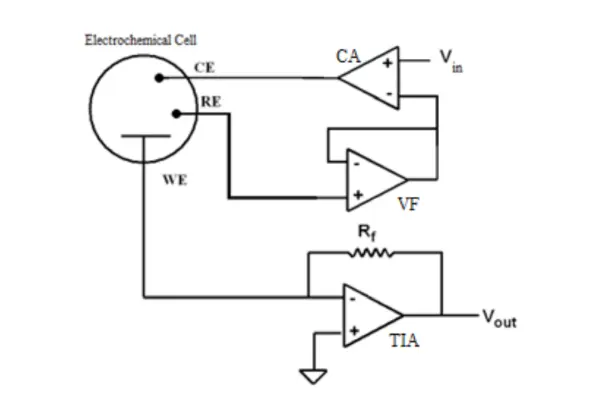
2 Methodology
The Arduino microcontroller boards, which are based on the ATMega microcontroller family, are renowned for their exceptional capabilities, affordability, and portability. Additionally, these boards offer digital outputs that can reach up to 5V, providing a range of ± 2.5V. This feature makes the boards suitable for producing the necessary output voltage range for conducting Electrochemical experiments when coupled with a voltage shifter circuit.
2.1 Potentiostat circuit design
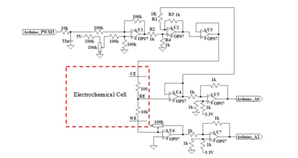
The Potentiostat Circuit depicted in Figure 2 draws inspiration from the potentiostat circuit proposed by [5]. However, significant differences exist between the two circuits. The major distinctions lie in the utilization of a single op-amp U1 for signal supply and shifting, which helps in minimizing the total number of op-amps required. Furthermore, instead of employing a ladder circuit to provide the signal from the I/O microcontroller ports to the potentiostat circuit, a straightforward RC filter has been introduced as an alternative approach.
2.2 Operation of the potentiostat
Pulse Width Modulation, commonly known as PWM, is a technique that enables achieving analog-like outcomes using digital methods. It involves digital control to generate a square wave, a signal that alternates between on and off states. By varying the duration of the on and off periods, this pattern can simulate voltages between full-on (5 Volts) and off (0 Volts).
However, in electrochemical measurements, it is preferable to have a DC-like signal with removed high frequencies. To achieve this, an RC filter has been introduced, comprising a resistance and a capacitor, as depicted in Figure 3. The RC filter is designed to effectively filter out high-frequency components, resulting in a smoother and more direct current-like signal for the electrochemical experiments.
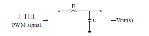
The RC filter’s cutoff frequency was calculated to be approximately 0.5Hz, resulting in a -60dB attenuation at the 1kHz frequency, which corresponds to the PWM signal frequency used.
Op-amp U1 functions as a Differential Amplifier (DA) and serves to drive the input signal from the Arduino PWM output. It adds an offset voltage value, derived from the voltage divider comprising 100K resistors and a 100K potentiometer at the non-inverting input, to shift the applied voltage to the cell within the desired range. The potentiometer allows the user to manually tune the applied voltage range according to their needs.
As mentioned earlier, Op-amp U2 takes on the role of the Control Amplifier. It compares the measured cell voltage with the desired voltage and drives current into the cell using an inverting configuration to provide negative feedback. This behavior can be mathematically described by the following equations: [Here you should include the relevant equations, as the current equations were mentioned in the original text, but they were not provided:
At the summing point,
????− = ????+ (1)
????− = ????+ = ???????????? (R4/????2 + ????4) (2)
If ???????????? = 0 ,
????′???????????? = (−????????????)????3/????1 (3)
If ???????????? = 0 ,
????′′???????????? = ???????????? (????4/????2 + ????4) (????1 + ????3/????1) (4)
Using the superposition theorem,
???????????????? = ????′???????????? + ????′′???????????? (5)
If all the resistors are of the same value, that is R1 = R2 = R3 = R4, then,
???????????????? = ???????????? − ???????????? (6)
the op-amp U2 becomes a unity gain differential amplifier
Op-amp U3 operates as a voltage follower, ensuring that the input signal remains isolated from the output, preventing any loading of the input. The voltage output from op-amp U3 is then connected to the CE.
Op-amp U4 serves as a voltage follower, fulfilling the function mentioned earlier for the Electrometer. Both Op-amp U5 and U7 act as voltage shifters, adding 3.3V from the Arduino to the output signals of the potentiostat, i.e., the measured voltage and current. This is necessary because the Arduino can only read voltage values from 0 to 5000 mV.
Consequently, the maximum applied voltage ranges that can be read by the potentiostat are determined to be from -3300 mV to +1700 mV. Although this range is not centered on 0V, it still encompasses most of the electrochemical application ranges.
Op-amp U6 functions as a transimpedance amplifier, serving the purpose described earlier for the TIA. The 10-100 kΩ gain potentiometer is utilized to read currents within the range from µA to mA, which corresponds to where most of the electrochemical reactions occur.
2.3 Simulation
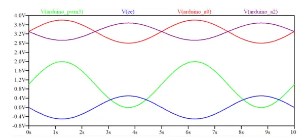
The LTspice simulator was employed to model the circuit presented in Figure 2. For simulation purposes, a sine wave source named “Arduino_PWM” was incorporated into the circuit’s input, imitating the triangular shape function typically employed in cyclic voltammetry. All op-amps used in the simulation were OP07, and they were powered with +9V and -9V in the rails.
Figure 4 exhibits the transient response of the circuit over a 10-second period. The input function is visualized as a green positive sine wave with an amplitude of 2 Vpp.
In order to center the input function (shown in green) at 0V, 1V was added using a voltage divider comprised of 100 kΩ resistors and a 100 kΩ potentiometer connected to the positive input of op-amp U1. The generated waveform applied to the cell through CE (V(ce), shown in blue) becomes inverted in comparison to the input signal due to the negative input signal inversion caused by the Differential Amplifier (U1).
The current sensed by WE is transformed into an inverted voltage value through the Transimpedance Amplifier (op-amp U6). This signal is then inverted again and 3.3V is added by the Differential Amplifier U7, sending the resulting signal to the Arduino Analog input (A2). The resulting wave, displayed in purple, is observed to be in phase with the input signal in blue.
Similarly, the voltage sensed by RE is sent to the Voltage Follower U4, which subsequently forwards it to the Differential Amplifier U5, converting it into an inverted value while adding 3.3V before being transmitted to the Arduino Analog input (A0). The resulting wave, depicted in red, is observed to be 180° out of phase with the input signal in blue, as expected.
2.4 Arduino software
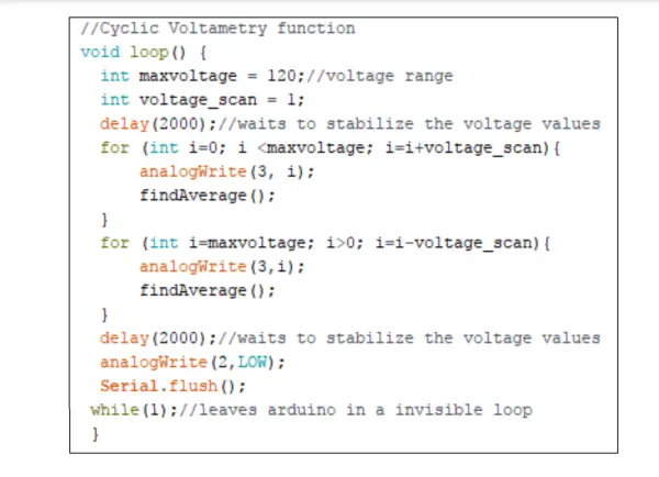
To execute Cyclic Voltammetry, it is necessary to apply a triangular-shaped output voltage curve to the Counter electrode. This scan is achieved by implementing a step function using two for loops: one for incrementing (forward direction of the cycle) and the other for decrementing (reverse direction of the cycle) the value in the analogWrite() function during each cycle, as depicted in Figure 5. The analogWrite() function adjusts the duty cycle of the PWM output pin, increasing and decreasing it respectively. Subsequently, the signal undergoes filtering and has an offset added by the potentiostat circuit before being applied to the Counter Electrode. The resulting output function is displayed in Figure 6.
The range of the applied voltage can be defined by adjusting the maxvoltage value.
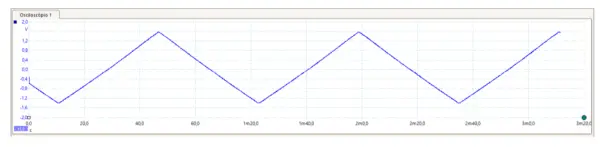
In Figure 6, the output voltage applied to the Counter Electrode during the execution of cyclic voltammetry function was measured using an oscilloscope (PicoScope 2000 series).
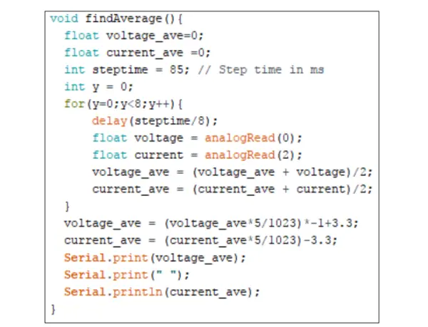
The findAverage() function, illustrated in Figure 7, reads 9 values in each step and computes both the average voltage and average current values. To eliminate the offset introduced by voltage shifter op amp U7, the current averaged value has 3.3V subtracted from it.
As the average voltage signal read is inverted by op amp U5, the value is then multiplied by -1 and 3.3V is added to obtain the actual voltage value.
It’s important to note that the calculated current value by the Arduino is actually a voltage value, which needs to be divided by the resistance of the TIA gain potentiometer to obtain the actual current measured at the working electrode.
By adjusting the steptime constant, one can change the duration of each step, effectively determining the scan rate of the cyclic voltammogram.
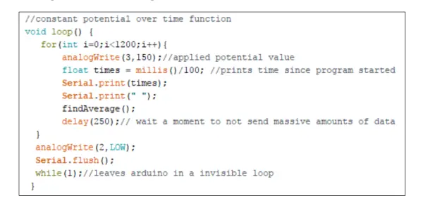
To facilitate specific electrochemical measurements, it can be advantageous to have a function that allows the user to easily control the duration of each step in the potential scan range. In pursuit of this objective, a constant potential over time function was developed, depicted in Figure 8.
This function applies an initial constant potential, and subsequently, the user can modify the applied potential by adjusting the potentiometer connected to U1, thus introducing an offset. Additionally, the function prints the elapsed time of the experiment, which is particularly useful for EC-SERS measurements conducted over time.
2.5 Processing software
During the execution of cyclic voltammetry, all the values measured by the Arduino Board are transmitted to the Serial port, where they can be observed in the serial monitor. However, it becomes valuable to store these values in a text file for further analysis. Additionally, real-time visualization of the cyclic voltammogram is quite useful for users to gain a better understanding of the ongoing electrochemical experiment.
To achieve this, the Processing software, an open-source programming software sketchbook, was utilized. Processing offers a Serial library that reads serial values from a USB port and a Print Writer library to create or open text files and print values into them. Furthermore, Processing provides functions to create windows for drawing geometric shapes.
The developed function creates a graph with the x-axis representing voltage and the y-axis representing current. It continuously reads the Serial values from a specified USB port in a cyclical manner, converting the values from strings to float numbers. These float numbers are then scaled to fit the graph’s axis using the map function, and subsequently, they are displayed on the graph in the drawing window and saved in a text file. The function continues this process until it has read the last value from the Serial port.
The code for this function is included in the Appendix.
2.6 Potentiostat circuit on a breadboard
The initial step involved in the potentiostat circuit development was assembling and testing it on a breadboard, illustrated in Figure 9.
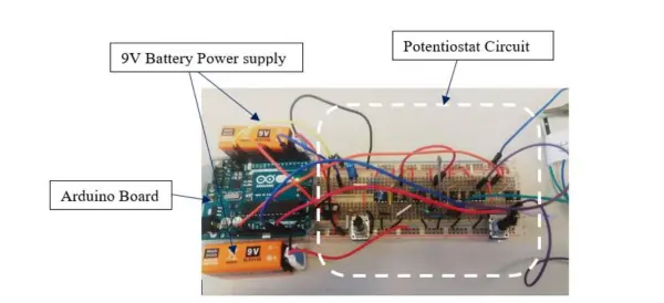
Utilizing the breadboard’s versatility for circuit development and testing, the potentiostat circuit underwent multiple iterations and adjustments before being transferred to a final copper strip board.
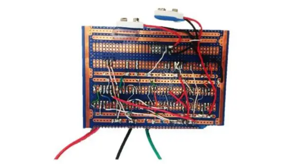
2.7 Transfer to an Arduino shield board format
In order to enhance the potentiostat’s compactness and durability, the circuit was migrated to a copper strip board. The components were soldered on the top side, while the connections were established by soldering wires on the back side of the board. You can observe this transformation in Figure 10.
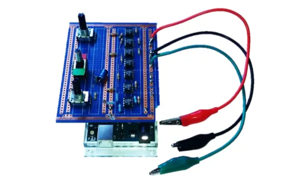
The Potentiostat board was designed to fit on top of the Arduino, and the connections were established using soldered pins, as illustrated in Figure 11.
2.8 Potentiostat testing and current resolution
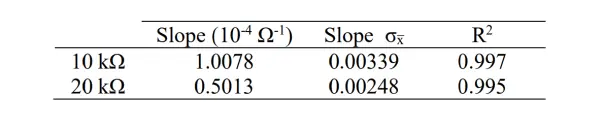
To assess the functionality of the fabricated potentiostat and verify its expected performance, 10 to 20 kΩ resistors were employed. The resistors’ well-known response serves as an excellent reference for evaluation, as the measured current responds linearly with a slope value of (1/R) when the voltage is varied.
To conduct the evaluation, the resistors were connected between the working electrode and reference electrode, simulating the cell resistance. Additionally, a small resistor (100 Ω) was connected between the reference and counter electrode to control the applied potential. A cyclic voltammetry (CV) of the resistors was recorded, and the resulting plot is depicted in Figure 12.
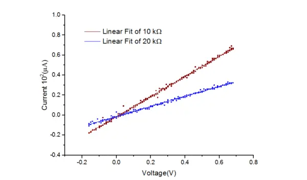
Based on the data presented in Table 1, the calculated resistance values were found to be 9.992 ± 0.033 kΩ and 19.948 ± 0.098 kΩ for the 10 kΩ and 20 kΩ resistors, respectively. These values exhibit a close alignment with the 5% tolerance of the resistors used.
The reference electrode voltage resolution was determined to be the minimum resolution of the measurement circuit, as calculated in equation 7.
10???????????? ???????????? ???????????????????????????????????????? =5000 ????????/210 = 4.8 ???????? ≈ 5???????? (7)
The current measurement is achieved through the transimpedance amplifier and the resistance Rf. The voltage drop across Rf is connected to one of the microcontroller’s ADC channels. To determine the current, Ohm’s law is implemented in the control software program based on the measured voltage and the value of Rf.
The resolution of the current measurement is dependent on both the voltage ADC resolution of the microcontroller, which is 5 mV as calculated in equation 7, and the value of Rf. The minimum detectable current by the potentiostat circuit can be calculated using Ohm’s law, as shown in equation 8.
Resolution =5 ????????/100 ???????? = 0.05 ???????? (8)
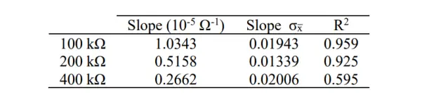
To experimentally evaluate the current resolution of the potentiostat, the maximum cell resistance that the potentiostat could accurately read without introducing significant errors was determined. The gain potentiometer in the Transimpedance Amplifier (TIA) was adjusted to its maximum value of 100 kΩ, and IV curves of 100 kΩ, 200 kΩ, and 400 kΩ resistors were measured. The results of these measurements are depicted in Figure 13.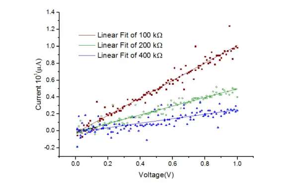
In the experiment, it is evident that as the resistance increases, the R-squared value (R2) decreases. However, with a cell resistance of 200 kΩ, the R2 value of the linear fit exceeded 0.9.
By utilizing the 200 kΩ resistor, the current was measured over time under various applied potentials, as depicted in Figure 14. It is noticeable that the current values can be differentiated from each other, despite the presence of considerable noise in the signals.
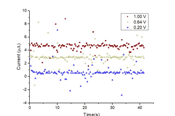
Although the calculated current resolution value was 0.05 µA, experimental results revealed that it fell within the range of 1 µA due to the presence of noise.
3 Electrochemical performance
3.1 Design of an electrochemical cell
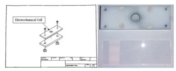
To facilitate electrochemical measurements, a straightforward Electrochemical Cell was devised, as depicted in Figure 15. The support structure consists of two rectangular-shaped slides, each with the dimensions of a standard glass slide, securely fastened together with screws. The central part of the upper slide forms the cell, which is round in shape. All components are made from non-conductive polymer material. To prevent any solution leakage, an o-ring with the same diameter as the cell was inserted between the slides.
3.2 Electrodes
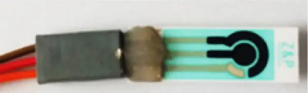
For the cyclic voltammetry measurements conducted in the developed electrochemical cell, Platinum and Carbon electrodes (acquired from Zimmer and Peacock) were utilized, as depicted in Figure 16. To establish contact between the wires and the screen-printed electrodes, silver paste was deposited and allowed to dry overnight. Subsequently, UV-curable glue was applied over the contacts to provide enhanced support and isolate each contact from one another.
3.3 Comparison with a commercial potentiostat
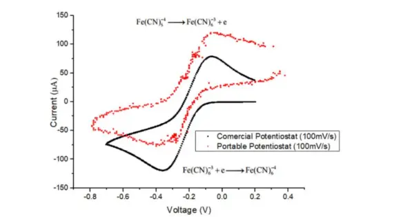
To assess the potentiostat’s performance, cyclic voltammetry was conducted using the standard reversible Ferricyanide-Ferrocyanide redox couple.
A comparison of the cyclic voltammetry results between the developed potentiostat and a commercial potentiostat (Ana Pot from Zimmer and Peacock company) is presented in Figure 17. Both potentiostats demonstrate oxidation and reduction peaks occurring at the same potentials, with the same peak current observed in both cyclic voltammograms. However, there is a consistent offset in the current measured between the two voltammograms. This offset can be attributed to a difference in the nominal resistance value of the 1 kΩ resistor, where 3.3 V are added in the Transimpedance Amplifier (TIA). While the code assumes that 3.3 V are added, a slight change in the resistor values can result in a different offset value from 3.3 V.
3.4 Diffusion coefficient determination
To demonstrate the capabilities of the potentiostat, cyclic voltammograms were conducted at various scan rates. These experiments allowed for the calculation of the diffusion coefficient of potassium ferricyanide in a solution with a known salt concentration using the Randles-Sevcik equation at a temperature of 25 °C:
???????? = 2.69 × 10^5 × ????^2/3 × ???? × ????^1/2× ????0 × ????^1/2 (9)
The Randles-Sevcik equation involves various parameters, including ‘n’ for the number of electrons transferred, ‘A’ representing the working electrode area in cm^2, ‘D’ denoting the diffusion coefficient in cm^2/s, ‘C0’ signifying the concentration in mol/cm^3, and ‘v’ representing the scan rate in V/s.
The Carbon working electrode used in the experiment had a diameter of 4 mm. The electrochemical cell was filled with a solution containing 5 mM potassium ferricyanide (from Sigma Aldrich) in 0.1 M NaCl (from Breckland Scientific Supplies Ltd). The potential was alternated between 0.35 V and -0.85 V at various scan rates, specifically 0.8, 0.11, 0.14, 0.25, and 0.35 V/s. The recorded data is illustrated in Figure 18.
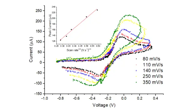
As anticipated, Figure 18 clearly demonstrates that the recorded electrochemical current increases as the scan rate rises. The inset plot illustrates the relationship between the anodic peak current and the square root of the scan rate, and as expected, it follows a linear pattern with a high R-squared value of 0.9993. By utilizing the Randles-Sevcik equation and calculating the slope of the linear fit, the diffusion coefficient of potassium ferricyanide is determined to be 4.3 × 10^-6 cm^2/s, which aligns well with the value found in the literature [6]. Any deviation between the calculated and literature values could be attributed to the previous calibration of the scan rates before conducting cyclic voltammetry experiments.
4 Conclusions and perspectives
The primary aim of this study was to design and evaluate a straightforward and budget-friendly potentiostat based on Arduino. It has been successfully demonstrated that this potentiostat can effectively carry out various electrochemical measurements, including cyclic voltammetry and potential step voltammetry. Additionally, the software allows for fine-tuning the scan rate of cyclic voltammetry measurements. The data acquisition is facilitated through the serial USB interface, enabling real-time display using the open-source processing software environment as a visual interface. Moreover, the acquired data can be saved in text file format for further analysis.
References:
[1] Kaswan, K. S., Singh, S. P., & Sagar, S. (2020). Role of Arduino in real-world applications. International Journal of Science and Technology Research, 9(1), 1113–1116.
Appendix
Processing code
import processing.serial.*;
Serial mySerial;
PrintWriter output;
void setup() {
mySerial = new Serial( this, "COM3", 9600 );//choose the USB port for serial
imput
output = createWriter( "data.txt" );//creates a text file in the same
directory of the Sketch
size(600, 400); // set the window size:
background(255);// set initial background
strokeWeight(2); // Default
line(40, 360, 580, 360);//x axis
line(40, 40, 40, 360);//y axis
line(40, 360, 40, 365);//x line lower limit
line(580, 360, 580, 365);//x line upper limit
line(302, 360, 302, 365);//0 line
textSize(15);
fill(0, 102, 153);
text("Voltage (V)", 285,390);//X axis label
fill(0, 102, 153);
text("-1.2", 30, 380);
fill(0, 102, 153);
text("0", 300, 380);
fill(0, 102, 153);
text("1.2", 575, 380);
fill(0, 102, 153);
rotate(-PI/2);
text("Current", -235, 30); // y axis label

}
//function that reads the serial values as strings and converts them in num
bers then it plots them and prints them on text file
void draw() {
if (mySerial.available() > 0 ) {
String value = mySerial.readStringUntil('\n');
if ( value != null ) {
println(value);
int p1 = value.indexOf(" ");
int l=p1-1;
String ss = value.substring(0, l+1);
String ss1 = value.substring(p1);
float voltage = float(ss);// convert to a number.
float current = float(ss1);// convert to a number.
println(voltage + " " + current);
output.println(voltage + " " + current);
float volt = map(voltage, -1.2, 1.2, 40, 580);//map to the screen width
float curr = map(current, -1, 1, 360, 40); //map to the screen height
ellipse(volt, curr, 3, 3);
}
}
}
//funtion to close the plot and save the file when any key of the keyboard
is pressed
void keyPressed() {
output.flush(); // Writes the remaining data to the file
output.close(); // Finishes the file
exit(); // Stops the program
}
- What is the main objective of the project?
To design, simulate, build, and test a low-cost Arduino-based potentiostat capable of electrochemical measurements like cyclic voltammetry and potential step voltammetry. - How does the potentiostat apply a DC-like voltage from the Arduino PWM output?
By using PWM with an RC filter (cutoff ≈ 0.5 Hz) to remove high frequencies and produce a smoother DC-like signal. - Can the Arduino read negative voltages from the potentiostat outputs?
Yes, signals are shifted by voltage shifter amplifiers (adding 3.3 V) so the Arduino can read voltages within 0–5000 mV, mapping applied ranges from −3300 mV to +1700 mV. - What amplifier stages are included in the potentiostat circuit?
The circuit includes a Control Amplifier (CA), Voltage Follower/electrometer (VF), Transimpedance Amplifier (TIA), differential amplifiers, and voltage shifters (U1–U7). - How is current measured by the potentiostat?
The TIA converts cell current at the working electrode into a voltage across Rf; the Arduino reads this voltage and software divides by Rf to obtain current. - What current resolution is theoretically and experimentally achievable?
Theoretical ADC voltage resolution is 5 mV giving a theoretical current resolution of 0.05 µA with Rf = 100 kΩ; experimentally noise limited resolution was about 1 µA. - How were the circuit and performance validated?
By LTspice simulation using OP07 op-amps and by experimental tests: measuring known resistors (10 kΩ, 20 kΩ) and comparing cyclic voltammograms with a commercial potentiostat using ferricyanide. - How is cyclic voltammetry implemented in the Arduino software?
By generating a triangular scan using two for loops that increment and decrement PWM duty cycle via analogWrite, with steptime determining step duration (scan rate). - How are data visualized and saved during experiments?
Arduino sends measured values over Serial USB to Processing software, which plots voltage vs current in real time and writes values into a text file. - What electrochemical cell and electrodes were used?
A simple polymer-based cell made from two glass-slide-sized polymer pieces with an o-ring; Platinum and Carbon screen-printed electrodes were used.