Summary of Brain-Computer Interface
The project developed a brain-computer interface using an AVR microcontroller to record EEG signals via passive electrodes and an analog amplification/filtering circuit. The digitized signals are transmitted through opto-isolated UART over USB to a PC, where MATLAB and C-based software perform FFT and machine learning (SVM) for signal analysis. This system enables control of a Pong game with brain waves and records sleep EEG data. Hardware includes an amplifier board, microcontroller, and an electrode cap based on the 10-20 system. Software utilizes MATLAB scripts and a real-time OpenGL plotter with FFT capabilities, integrating neurofeedback through P300 detection and brainwave classification.
Parts used in the Brain-Computer Interface:
- AVR Microcontroller
- AD620 Instrumentation Amplifier
- 3140 Operational Amplifier
- Silver-plated Passive EEG Electrodes
- Fairchild Semiconductor 6N137 Optoisolator
- FTDI USB UART Chip
- 4 AA Batteries (+6 VDC power supply)
- Old Baseball Cap (for EEG electrode placement)
- Digi-Key Electronic Components
- Samples from Analog Devices, Texas Instruments, Maxim Semiconductor
- MATLAB Software
- OpenGL and C++ Software with FFTW and SDL libraries
Introduction
Our goal was to build a brain-computer interface using an AVR microcontroller. We decided that the least invasive way of measuring brain waves would be using electroencephalography (EEG) to record microvolt-range potential differences across locations on the user’s scalp. In order to accomplish this, we constructed a two-stage amplification and filtering circuit. Moreover, we used the built-in ADC functionality of the microcontroller to digitize the signal. Passive silver-plated electrodes soaked in a saline solution are placed on the user’s head and connected to the amplifier board. The opto-isolated UART sends the ADC digital values over USB to a PC connected to the microcontroller. The PC runs software written in MATLAB and C to perform FFT and run machine learning algorithms (SVM) on the resultant signal. From there, we were able to control our own OpenGL implementation of the classic PC game Pong using our mind’s brain waves. We also wrote software to record our sleep and store the EEG signal inside a data file.

High-Level Design
Rational and Inspiration for Project Idea
Our project idea was inspired by Charles’s severe obstructive sleep apnea (OSA) disorder. In order to diagnose sleep apnea, a clinical sleep study is performed where the patient is attached to EEG electrodes, along with SpO2, EMG, and respiration sensors. The patient’s sleeping patterns are recorded overnight, and apneas (periods of sleep without breathing) can be identified within the collected data. This process is costly and requires an overnight stay at a hospital or sleep lab. Moreover, the patient often is denied access to their own data since a licensed sleep specialist interprets it for them. Our goal was to build a low-cost alternative that would allow users to take their health in their own hands by diagnosing and attempting to treat their own sleep disorders. Moreover, our project has diverse applications in the areas of neurofeedback (aiding meditation and treatment of ADHD disorder), along with brain-computer interfaces (allowing the disabled to control wheelchairs and spell words on a computer screen using their thoughts).
Background Math
Support Vector Machines
The machine learning algorithm we used was a support vector machine (SVM), which is a classifier that operates in a higher dimensional space and attempts to label the given vectors using a dividing hyperplane. The supervised learning method takes a set of training data and constructs a model that is able to label unknown test data. A brief explanation of the mathematics behind SVMs follows. During training, the SVM is given a set of instance-label pairs of the form {(xi⃗ ,yi):i=1,…,l} where the instances are n-dimensional vectors such that xi⃗ ∈Rn. The n dimensions represent n separate “features.” In addition, the labels are in the form y∈{1,−1}, where 1 and -1 designate target and non-target instances respectively. To “train” the support vector machine to recognize unknown input vectors, the following minimization problem is solved:
subject to:
Source: http://www.csie.ntu.edu.tw/~cjlin/papers/guide/guide.pdf
Note that ϕ is a function that maps the training vectors x⃗ i into a higher-dimensional space, while C>0 and ξi act as error terms (so-called “slack variables”). Moreover, K is the kernel function which is defined as K(ϕ(xi)Tϕ(xj)). For our purposes, we used a radial basis function (RBF) kernel which has a K function of K(xi,xj)=exp(−γ||xi−xj||2) where γ>0 represents a user-tunable parameter.
DFT
The discrete Fourier transform (DFT) transforms a sequence of N complex numbers (an N-point signal) in the time-domain into another N-sequence in frequency domain via the following formula:
The Fourier transform is denoted by F, where X=F(x). Source: http://en.wikipedia.org/wiki/Discrete_Fourier_transform
An algorithm, the Fast Fourier Transform (FFT) by Cooley and Tukey, exists to perform DFT in O(nlogn) computational complexity as opposed to O(n2). We take advantage of this speed-up to perform DFTs in real-time on the input signals.
Filters
In order to filter the brain wave data in MATLAB, we use a finite impulse response (FIR) filter which operates on the last N+1 samples received from the ADC. In signal processing, the output y of a linear time-invariant (LTI) system is obtained through convolution of the input signal x with its impulse response h. This h function “characterizes” the LTI system. The filter equation in terms of the output sequence y[n] and the input sequence x[n] is:
Note that only N coefficients are used for this filter (hence, “finite” impulse response). If we let N→∞, then the filter becomes an infinite impulse response (IIR) filter. Source: http://en.wikipedia.org/wiki/FIR_filter
EEG Signal Analysis
The EEG signal itself has several components separated by frequency. Delta waves are characteristic of deep sleep and are high amplitude waves in the frequency range 0≤f≤4 Hz. Theta waves occur within the 4-8 Hz frequency band during meditation, idling, or drowsiness. Alpha waves have frequency range 8-14 Hz and take place while relaxing or reflecting. Another way to boost alpha waves is to close the eyes. Beta waves reside in the 13-30 Hz frequency band and are characteristic of the user being alert or active. They become present while the user is concentrating. Gamma waves in the 30-100 Hz range occur during sensory processing of sound and sight. Lastly, mu waves occur in the 8-13 Hz frequency range while motor neurons are at rest. Mu suppression takes place when the user imagines moving or actually moves parts of their body. An example diagram of the EEG signal types follows:
EEG signals also contain event-related potentials (ERPs). An example is the P300 signal, which occurs when the user recognizes an item in a sequence of randomly presented events occurring with a Bernoulli distribution. It is emitted with a latency of around 300-600 ms and shows up as a deflection in the EEG signal:
Other artifacts present themselves in the EEG signal as well such as eye blinking and eye movement. An illustration of an example signal corrupted by eye blinking follows:
Logical Structure
The overall structure of the project consists of an amplifier pipeline consisting of a differential instrumentation amplifier (where common-mode noise is measured using a right-leg driver attached to the patient’s mastoid or ear lobe), along with an operational amplifier and some filters (to remove DC offsets, 60 Hz power-line noise, and other artifacts). From there, the signal passes to the microcontroller, where it is digitized via an ADC. Next, it is send over an isolated USB UART connection to a PC via an FTDI chip. The PC then performs signal processing and is able to output the results to the user, creating a neurofeedback loop which allows the user to control the PC using their brain waves. A functional block diagram of the overall structure follows:
Hardware/Software Trade-offs
Performing FFT in hardware using a floating-point unit (FPU) or a field programmable gate array (FPGA) would have allowed us to realize a considerable speed-up; however, our budget was only limited to $75, so this was not an option. Another trade-off we encountered was the use of MATLAB versus C. MATLAB is an interpretted language whose strength lies in performing vectorized matrix and linear algebra operations. It is very fast when performing these operations, but it is an interpreted language that does not run as native code. This speed penalty affected us when we attempted to collect data in real-time from the serial port at 57600 baud. To combat this speed penalty, I wrote a much faster OpenGL serial plotting application in C that runs at 200-400 frames per second on my machine (well above the ADC sample rate of 200 Hz) and is able to perform FFTs in real-time as the data comes in. Furthermore, yet another trade-off was the decision to use the PC to output the EEG waveforms rather than a built-in graphical LCD in hardware. Once again, budget constraints limited us, along with power usage since for safety reasons, our device uses four AA batteries instead of a mains AC power supply.
Relationship of Your Design to Available Standards
There exists a Modular EEG serial packet data format that is typically used to transmit EEG data over serial; however, we used ASCII terminal output (16-bit integer values in ASCII separated by line breaks) for simplicity, ease of debugging, and compatibility with MATLAB. Moreover, serial communications followed the RS232/USB standards. Another consideration was the IEC601 standard. IEC601 is a medical safety standard for medical devices that ensures that they are safe for patient use. Unfortunately, testing for IEC601 compliance was very much out-of-budget. Nevertheless, we discuss the many safety considerations that we absolutely adhered by in the Safety subsection (under Results) of this report.
Hardware Design
Amplifier Board Design
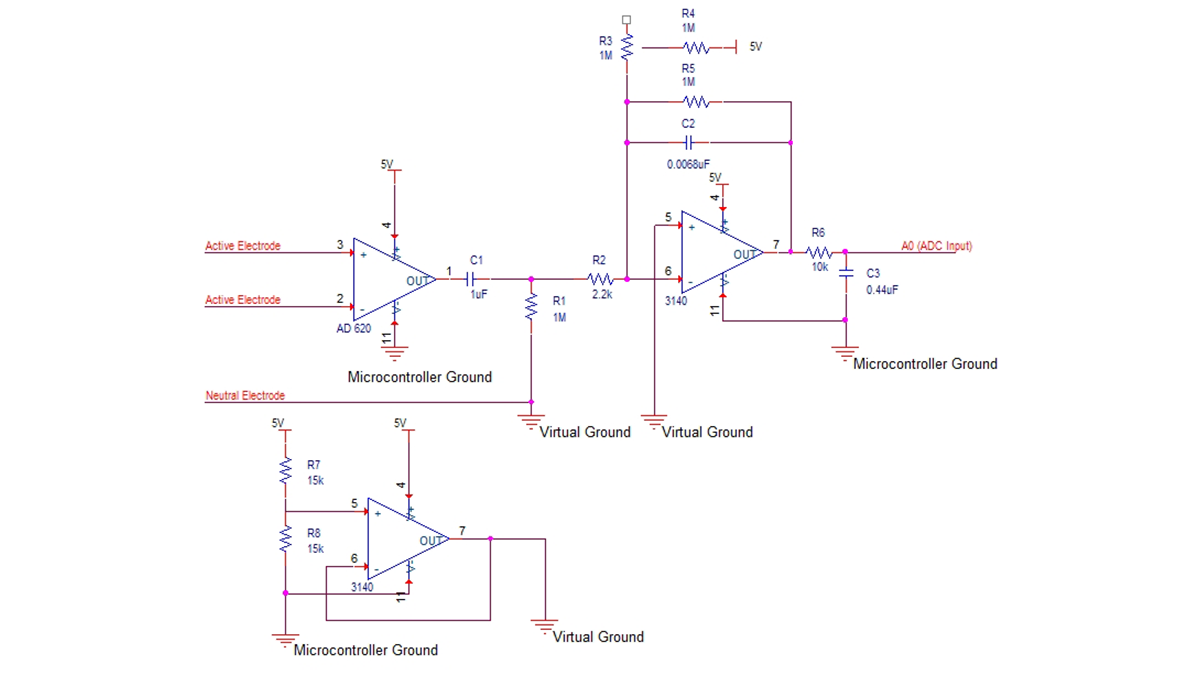
We built an analog amplification circuit with a total gain of 1,500 based on the design by Chip Epstein at https://sites.google.com/site/chipstein/home-page/eeg-with-an-arduino with modified gain and filter stages. The first stage uses an AD620 instrumentation amplifier for differential common mode signal rejection to reduce noise. The gain of the AD620 is approximately 23. A voltage divider and a 3140 opamp buffer provide a 2.5 V virtual ground for the instrumentation amplifier. After passing through the instrumentation amplifier, the signal is filtered using an RC high pass filter with fc=0.13 Hz (we modified the original design to allow the P300 ERP to reside within the pass-band of the filter).
Next, the signal undergoes a second-stage amplification. The gain of a 3140 opamp is set to approximately 65. The output signal is then filtered using an RC low-pass filter with a cut-off frequency of approximately 48 Hz. This frequency was chosen to preserve the low-frequency content of the EEG signal, while removing 50-60 Hz power line noise from the signal. We ordered parts from Digi-Key and samples from Analog Devices, Texas Instruments, and Maxim Semiconductor. We also sampled silver-plated passive EEG electrodes. From there, we were able to amplify a 125 μVVpp, 10 Hz square wave calibration signal to well within the ADC reference voltage range (0-1.1 V) and plot it on a PC in real-time. We constructed this prototype circuit on a breadboard. A schematic diagram of the amplifier board follows:
Microcontroller Board Design
The microcontroller board contains a voltage divider that outputs a 125 μVVpp, 10 Hz square wave calibration signal from Pin D.3 of the microcontroller. Moreover, it contains a +6V DC battery-power supply that provides DC power to the microcontroller and the amplifiers. A schematic diagram of the microcontroller board follows:
Opto-Isolated UART over USB Design
We constructed an isolated +6 VDC power supply using 4 AA batteries and connected it the microcontroller using the PCB target board. We cut the ground trace connecting the microcontroller ground to the USB ground using a dremel tool. An illustration of the cut that we performed follows:
We used a Fairchild Semiconductor 6N137 optoisolator to isolate the USB power from the microcontroller power. The line of isolation is between the microcontroller UART RX and TX pins (Pin D.0 and Pin D.1) and the FTDI chip’s RX and TX pins. A schematic diagram of the isolation circuit follows:
Electrode Cap Design
We constructed an EEG helmet consisting of an old baseball cap modified to contain EEG electrodes. We followed the International 10-20 System of Electrode Placement by including electrodes at the designated locations on the scalp: Occipital lobe (O), Central lobe (Fz, Pz, C3, C4, Cz), and Frontal lobe (Fp1, Fp2, G). A diagram of the 10-20 system of electrode placement follows:
Software Design
MATLAB Serial Code
The primary function of the MATLAB serial code is to acquire digital EEG signal data from the microcontroller over the serial port. We wrote some code to plot the signal onto the screen and to perform rudimentary signal processing tasks (FFT and filtering). The MATLAB code consists of three files: plot_samples.m, plot_samples_rt.m, and serial_test.m
The serial_test.m script opens the serial port and displays an almost real-time plot of the serial data. It parses the serial data in a while loop via fscanf and str2num. Additionally, it updates the plot window contents using MATLAB’s drawnow command. The loop terminates if the user closes the plot window, causing the script to clean up the file handle and close the serial port.
The plot_samples.m script opens the serial port, and reads exactly N=200 samples of EEG data (around 2 seconds). It then closes and cleans up the serial port. Next, a 60 Hz notch filter is applied to the signal to remove powerline noise via the iirnotch and filter, and the DC offset (mean value) is subtracted from the signal. Finally, the time-domain signal is displayed in a plot window, along with the single-sided amplitude spectrum computed via MATLAB’s fft function.
The plot_samples_rt.m script performs exactly the same operations as the plot_samples.m script, except it performs them in a loop. The script operates by sampling N=200 samples repeatedly until the user closes the plot window. As an effect, the signal plot and the frequency spectrum are refreshed every 2 seconds giving psuedo real-time operation.
OpenGL Plotter
A real-time serial plotter was written in OpenGL and C++. OpenGL is a high-performance graphics library, while C++ is much faster than MATLAB since it runs as native code. The program displays the real-time wave form from the serial port, along with its FFT. We use the FFTW (Fastest FFT in the West) library for computing the FFT using fast algorithms. Moreover, extensions were later added to the plotting code allow Pong to be played using brain waves, along with a P300 ERP detector. A data logging feature was added to allow us to record our EEG data while asleep to a file. The SDL library is used to collect user input from the keyboard and output the OpenGL graphics buffer to an on-screen window.
Initialization and Event Loop
The main() function initializes the SDL library, clears the ADC buffers, initializes OpenGL, initializes SDL TTF (for True Type font rendering), opens the serial port, opens the log file, and initializes the FFTW library. From there, the program enters the main event loop, an infinite while loop which checks for and handles key presses, along with drawing the screen via OpenGL.
The Quit() function cleans up SDL, closes the serial port, de-initializes FFTW frees the font, and quits the program using the exit UNIX system call.
The resizeWindow() function changes the window size of the screen by changing the viewport dimensions and the projection matrix. For this project, we use an orthographic projection with ranges x∈[0,X_SIZE] and y∈[0,ADC_RESOLUTION]. The handleKeyPress() function intercepts key presses to quit the game (via the [ESCAPE] key) and to toggle full screen mode (using the [F1] key).
The initGL() function initializes OpenGL by setting the shading model, the clear color and depth, and the depth buffer.
Drawing Code
The drawGLScene() function is called once per frame to update the screen. It clears the screen, sets the model view matrix to the identity matrix I4, shifts the oscilloscope buffer running_buffer to the left by one, and fills the new spot in the buffer with the newest sample from the serial port. This sample is obtained by calling the readSerialValue() function in serial.cpp. This function also contains logic to perform the FFT and draw it onto the screen as well. The sample is sent to the P300 module and logged to the output file. Moreover, the power spectrum of the FFT is computed using rfftw_one() and by squaring the frequency amplitudes.
The FFT bars and the oscilloscope points are plotted using GL_LINES and GL_POINTS respectively. Moreover, lines join adjacent oscilloscope points. The frequency ranges corresponding to each brain wave classification (alpha, beta, etc.) are calculated, along with their relative powers. Moreover, BCI code is executed which will be discussed in the OpenGL Pong sub-section of this report. The pong and P300 modules are then drawn on the screen, along with status text using TTF fonts and the framebuffer is swapped. Lastly, the frame rate is calculated using SDL_GetTicks(), an SDL library function.
Serial Code
The serial code handles serial communications over USB and is located in serial.cpp. Important parameters such as the buffer size BAUD_RATE, the port name PORT_NAME, and the baud rate B57600 are stored as pre-processor directives. The openSerial() function opens the serial port and sets the baud rate to 57600 (56k). The readSerialValue() function reads and parses one 10-bit ASCII ADC value from the serial port by scanning for a new-line terminator and using sscanf (readByte() is unused). Lastly, the closeSerial() function closes the serial port device. The UNIX system calls open, read, and close are used to carry out serial I/O, along with the GNU C library’s system() function. The device file name for USB serial in UNIX is /dev/ttyUSB0.
Note that if the NULL_SERIAL pre-processor directive is set, then mock serial data is used rather than actually collecting data from the serial device. This functionality is useful for testing purposes.
Configuration
The config.h file contains pre-processor directives that can be used to configure the OpenGL plotting application during compile-time. Important parameters include the screen width and height (SCREEN_WIDTH and SCREEN_HEIGHT respectively), the screen bit depth (SCREEN_BPP), ADC_RESOLUTION the ADC resolution (the number of y-values) set to 210=1024, and the log file name LOG_FILENAME (defaulting to "eeg_log.csv").
Debugging
Useful utility functions for debugging purposes are found in debug.cpp. The FileExists() function returns a boolean indicating whether the given file exists. The OpenLog() and CloseLog() functions are useful for writing log files with time and date stamps. The log_out() function can be passed a format string which is written to the log file, along with a time stamp. The format() function takes a format string and returns the formatted result. It uses the vformat utility function to generate the format string based on the arguments passed to the function. The dump() function dumps regions of memory to the screen in a human-friendly hexadecimal format.
Font Rendering
TTF font rendering support was implemented using NeHe sample code (located in the References section of this report). The glBegin2D() and glEnd2D() functions set up an orthographic screen projection for font rendering. Meanwhile, power_of_two() is a utility function that calculates the next largest power-of-two of the given integer input (useful for computing OpenGL texture dimensions which must be powers of two). The SDL_GL_LoadTexture() function converts an SDL_Surface structure in memory to an OpenGL texture object. This is useful because the SDL_TTF library only returns an SDL_Surface, but we are rendering the fonts using OpenGL. The InitFont() and FreeFont() functions use the SDL_TTF library functions to load and free fonts respectively. Lastly, glPrint() acts like an OpenGL implementation of printf by printing strings to the screen using TTF font textures in SDL_TTF.
For more detail: Brain-Computer Interface