Required Equipment
- lightbulb (incandescent, LED, CFL, etc.)
- AC solid-state relay (hockey-puck type, etc.)
- temperature sensor (TMP36, etc.)
- Arduino board (e.g. Uno, Mega 2560, etc.)
In this example, the temperature of the lightbulb is gauged using a TMP36 sensor. This sensor is cost-effective, reasonably accurate, and encompasses a sufficient range. The Arduino board serves the dual purpose of powering the sensor and interpreting the sensor’s output through an Analog Input. Additionally, the Arduino board generates the Digital Output that regulates the activation and deactivation of the solid-state relay. This digital output establishes intermittent connections and disconnections between the light bulb and the AC power source (from the wall) via the relay, facilitating the switching on and off of the light bulb. The control logic employed to determine the relay’s activation and deactivation instances is programmed in Simulink, which is also utilized to visually represent both the lightbulb’s temperature and the control signal.
Objective
The intention behind engaging in this exercise involving the lightbulb is to exemplify the control of switched systems. By turning the lightbulb on, its temperature increases, and conversely, turning it off leads to a decrease in temperature (within environmental boundaries). The lightbulb operates as a binary system, confined to two states: on or off. It either remains connected to the AC source or is disconnected; its luminosity cannot be adjusted. In this experiment, we observe the resultant “chattering” behavior of the lightbulb and explore alternative approaches aimed at mitigating the frequency of this chattering phenomenon or refining its fluctuations. This is accomplished through the application of dead bands, low-pass filters, and Pulse-Width Modulation. Furthermore, this activity facilitates exposure to Proportional (P) control, Proportional-Integral (PI) control, and first-order systems.
System identification experiment
To establish our temperature control system, a formal plant model (the lightbulb) might not be strictly necessary. Instead, we can adopt a logical approach that activates the lightbulb when the measured temperature dips below the desired level, and deactivates it when the temperature surpasses the desired threshold. Nevertheless, our intention is to elucidate the resultant behavior of our control system and possibly refine the control algorithm with a higher degree of intelligence. Hence, we aim to formulate a model for the lightbulb’s thermal dynamics grounded in its observed response. This form of model is occasionally referred to as a black box model or a data-driven model. Once we develop such a model, our endeavor extends to explaining our observations through an understanding of the fundamental physics at play.
Hardware setup
Within this experiment, our chosen system is a conventional incandescent lightbulb, and our ultimate objective is to regulate the temperature of this lightbulb. To align with the capabilities of the selected temperature sensor, we opted for a 25 W bulb, ensuring that the maximum temperature remains within the confines of the sensor’s range. Furthermore, you have the flexibility to utilize different bulb variants (LED, CFL, etc.) as well.
In our temperature measurement setup, we will utilize the TMP36 sensor, although various other options are also available. This sensor gauges temperature in Celsius and is remarkably cost-effective, priced at just a few dollars. It offers a suitable range, reasonable precision, and the added advantage of not requiring calibration. Notably, the TMP36 sensor is frequently included in numerous Arduino starter kits available in the market. The datasheet for this sensor can be accessed here. To affix the temperature sensor to the lightbulb’s surface, you can opt for thermally conductive epoxy or adhesive metal tape. Connecting the TMP36 to the Arduino Board involves the following arrangement. If the sensor is positioned such that the pins point downward and the flat side faces you, the leftmost pin corresponds to power (within the range of 2.7 V to 5.5 V), the middle pin functions as the signal interface, and the rightmost pin is for ground. Power and ground for the TMP36 are supplied by the Arduino board, while the signal—presenting a voltage that maintains a linear proportionality with temperature—is read using one of the board’s Analog Inputs.
To initiate the lightbulb’s activation and deactivation, a digital output signal is employed from the Arduino board, facilitated by a solid-state relay. Essentially, this relay functions as an electrical switch capable of connecting or disconnecting a device (which could potentially have high power requirements) to an AC source using a low-power DC signal. In our context, the AC source originates from a standard wall outlet, while the DC signal is supplied by a Digital Output signal from the Arduino board. Consequently, our solid-state relay must be equipped to manage 120-240 V on the AC side (in North America, 120 V is required), with the DC side controllable by a 5 V signal.
Given that our load, which is the lightbulb, is resistive in nature (not inductive) and doesn’t demand substantial current, the choice of solid-state relay need not be overly meticulous. In our case, we are opting for a straightforward “hockey-puck” style relay. To govern the lightbulb’s operation, the relay needs to be inserted into the circuit (the loop) that connects the lightbulb to the wall outlet. This necessitates modifying the cord for the lightbulb and integrating the relay into the circuit. While undertaking this task, ensure that the lightbulb is not plugged in. The insertion of the relay should occur on the neutral wire of the lightbulb’s plug. The neutral wire can be identified by a white stripe or ribbing. Placing the relay on the live wire will result in the relay’s terminals being connected to the power supply even when the relay is in the off state. Furthermore, remember to adequately cover the exposed relay terminals and refrain from touching the terminals when the lightbulb is plugged in.

Software setup
Within this experiment, we will utilize Simulink to instruct the relay, retrieve data from the temperature sensor, and generate real-time data visualization. Specifically, we will utilize the IO package offered by Math Works for this purpose. If you require guidance on utilizing the IO package, you can refer to the provided link. Additionally, we will illustrate how to integrate the control logic directly into the Arduino board.
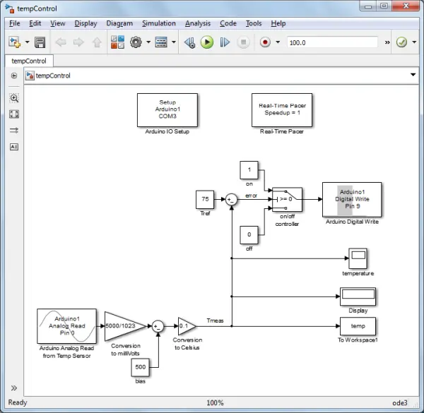
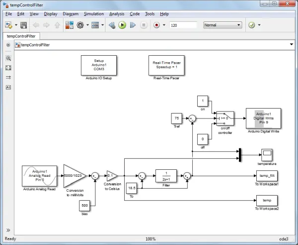
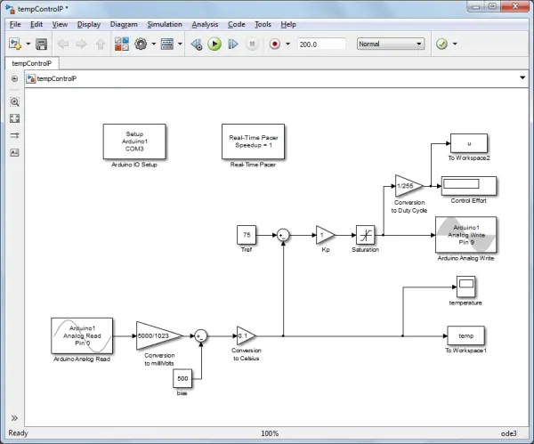
The Simulink model that we will utilize is provided below and can be downloaded from this link. If necessary, you may need to modify the COM port in the IO Setup block to correspond with the location where your Arduino board is connected. Within this model, the temperature data is acquired through an Analog Read on channel A0. Subsequently, this data is converted from counts to degrees Celsius. The raw temperature data is presented in bits, as the Arduino Board incorporates a 10-bit analog-to-digital converter. This signifies that by default, an Analog Input channel reads a voltage ranging from 0 to 5 V, dividing this interval into 2^{10} = 1024 increments. Hence, an output of 0 corresponds to 0 V, while an output of 1023 corresponds to 5 V.
Given that the TMP36’s maximum output voltage is 1.75 V, utilizing the on-board 3.3 V source for AREF instead of the default 5 V provides improved resolution. The data in bits is then transformed to millivolts (assuming a default 5 V reference), followed by conversion to temperature in degrees Celsius. This final conversion is grounded in the information found in the TMP36’s datasheet. The model then visually exhibits the stored data through a scope and a display, and this data is also recorded in the MATLAB workspace for subsequent analysis.
Within this model, the relay’s operation is directed to be open (1) or closed (0), which aligns with the lightbulb’s state of being on or off, through a Digital Write on channel 9. To initiate, we will employ a step input, wherein the lightbulb is initially off and is subsequently switched on.
The components contributing to this functionality include the Arduino Analog Read block, Digital Write block, IO Setup block, and Real-Time Pacer block, all integrated within the IO package. The remaining blocks originate from standard Simulink libraries, specifically, they are accessible in the Math, Sinks, and Sources libraries.
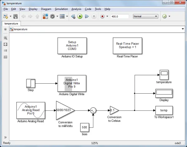
By double-clicking on the Analog Read block, we have the option to modify the “Sample time.” The optimal sampling rate for the system while ensuring real-time communication and Simulink plotting is around 0.01 seconds. Sampling at a faster rate could lead to the Simulink model operating slower than real-time, rendering it unable to meet the specified sampling rate.
Given the relatively gradual thermal dynamics of the lightbulb, a sample time of 0.1 proves to be more than satisfactory. This identical value for the sample time will be set within the Digital Write block as well.
After constructing the Simulink model, it can be executed to gather a dataset similar to the one illustrated below. In the beginning, the lightbulb starts at the room temperature when the model is initiated. At t = 50 seconds, the lightbulb is switched on using the step input, commencing its heating process. To ensure accurate estimation of the initial lightbulb temperature (ambient temperature), we allow 50 seconds before activating the lightbulb. It’s essential to execute the model for a considerable duration to allow the lightbulb’s temperature to stabilize at a steady state.
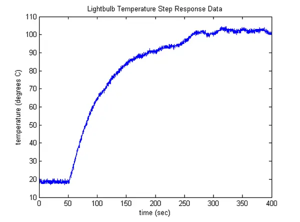
Upon analyzing the provided response data, it becomes apparent that the thermal behavior of the lightbulb exhibits characteristics resembling a first-order system. Leveraging this observation, we will utilize this property to formulate a model for the lightbulb’s behavior.
Modeling
In this experiment, our approach involves developing a model for the lightbulb’s thermal dynamics using only the step response data we have collected. This means that we will create a model based solely on the recorded data without delving into the fundamental physics underlying the system. By analyzing the collected data, it’s evident that the thermal behavior of the lightbulb follows an approximate first-order pattern. Thus, we aim to create a fitting transfer function for the data, as depicted below, where $K$ represents the system’s DC gain and $\tau$ symbolizes the system’s time constant.
![]()
In the context of our specific lightbulb system, we will define the input as the percentage of time the lightbulb is switched on, denoted as the duty cycle D(s). Correspondingly, the output we will focus on is the difference in temperature ΔT(s) between the lightbulb’s temperature T and the ambient temperature To. We have opted for ΔT as the output choice, rather than solely T, to achieve a linear model. To adhere to the principle of a linear system, the output should exhibit a linear relationship with the input. This implies that an input of 0 should result in an output of 0.
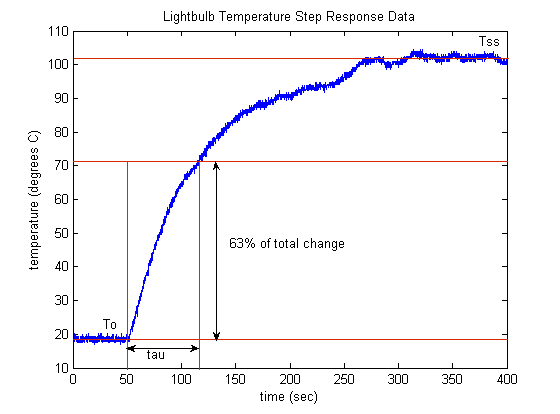
Upon analyzing the provided data, a few challenges arise when attempting to estimate the parameters K and tau due to signal noise and data drift. Noise’s influence can be mitigated through techniques such as low-pass filtering or smoothing the data. In this instance, we’ll take a more informal approach and visually approximate an averaged curve from the data. The data drift, which could be attributed to factors like fluctuations in ambient temperature, convection currents, voltage amplitude variations, sensor inaccuracies, etc., can similarly be accounted for by approximating an average across the variations.
Upon analyzing the provided step response data, it can be deduced that the initial ambient temperature (initial lightbulb temperature) is approximately 18.5 degrees Celsius, while the lightbulb’s steady-state temperature settles around 102 degrees Celsius. As the input corresponds to a full 1 (100 percent duty cycle) and the output is represented by ΔT, this implies that the system’s DC gain K is roughly 83.5 degrees Celsius (102 – 18.5). Utilizing the definition of the time constant as the period required for the system response to reach 63% of its total alteration, the estimated time constant for this system stands at approximately 66 seconds. Referencing the annotated version of the step response plot below, it’s evident that 0.63 multiplied by 83.5 degrees plus 18.5 degrees equates to around 71.1 degrees, which corresponds to approximately 116 seconds. Given that the step input occurred at 50 seconds, this infers a time constant of approximately 66 seconds (116 – 50).
Considering the parameter identification described above, the resultant estimated model for the thermal dynamics of the lightbulb is as follows.
![]()
To assess the degree of fit between our derived model and the collected data, we will execute the subsequent MATLAB commands. Here, the output of our previous Simulink model, labeled as “temp,” is stored as a timeseries.
   s = tf('s');
         To = 18.5;            % ambient/initial temperature
         K = 83.5;             % DC gain
         tau = 66;             % time constant
         P = K/(tau*s+1);      % model transfer function
         [y,t] = step(P,350);  % model step response
         plot(t+50,y+To);
         hold
         plot(temp,'r:')
         xlabel('time (sec)')
         ylabel('temperature (degrees C)')
         title('Lightbulb Temperature Step Response')
         legend('model','experiment','Location','SouthEast')
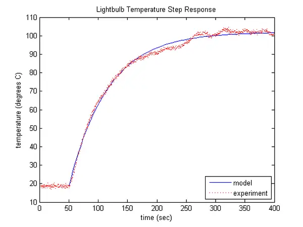
Upon analyzing the information presented above, it becomes evident that our choice of a first-order model appears to be well-founded. This alignment with our assumption is not unexpected, especially when we delve into the fundamental physics of the lightbulb. By delving into the heat equilibrium of the lightbulb, we can outline the following:
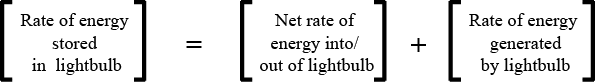
Taking into account that the speed at which energy is stored relies on the light bulb’s “thermal capacitance,” and the overall pace of heat transfer is determined by the light bulb’s thermal conductivity (akin to the reciprocal of “thermal resistance”) along with the disparity between the bulb’s temperature and the ambient temperature, while considering the heat generation as the system’s input (likely resembling an almost perfect step due to the rapid electrical dynamics), we can establish the following fundamental equation governing the behavior of the system.
![]()
Rewriting the above in terms of  , we can make use of the fact that
  is approximately constant, that is
  , which leads to the following.
![]()
Examining the provided content reveals that the thermal behavior of the lightbulb can be characterized by a first-order differential equation, the behavior of which mirrors that of an RC circuit, with the time constant 𝜏=RC
ON/OFF Control
Having gained an understanding of the plant’s behavior and established a model, we can now explore control strategies. Our initial approach to control involves an ON/OFF controller aimed at regulating the lightbulb’s temperature. This controller activates the lightbulb when the measured temperature is below the desired temperature (error > 0), and deactivates it when the measured temperature exceeds the desired temperature (error < 0). To implement this logic, we’ve adjusted the Simulink model by employing a Switch block with a reference temperature of 75 degrees Celsius. The modified model is available for download here.
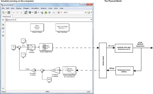
The control strategy depicted above operates without utilizing any insight from the plant model and relies on feedback. Visualizing the feedback loop can be challenging due to the plant’s presence in the real world. The illustration below aids in clarifying how the complete feedback system, comprising the Simulink model and the physical realm, aligns.
Let’s pause for a moment to consider how you might establish an open-loop controller for this system (without directly measuring the lightbulb’s temperature) using the model we derived earlier. What potential benefits and drawbacks would be associated with such an approach?
The temperature response of our lightbulb under the closed-loop ON/OFF controller is displayed below. The behavior is quite intuitive. Initially, the lightbulb is too cold, prompting the controller to activate the bulb. As a result, the bulb starts to heat up. After around 75 seconds, the lightbulb’s temperature nearly reaches the target of 75 degrees Celsius, causing the controller to deactivate the bulb. As the bulb releases heat to its surroundings, its temperature declines until it falls below 75 degrees, triggering the bulb to be turned on again. Consequently, this ON/OFF control strategy leads to the lightbulb flickering, undergoing rapid on-off cycles, and causing the temperature to oscillate around the desired value. The presence of noise in the measured temperature signal can further amplify this flickering effect.
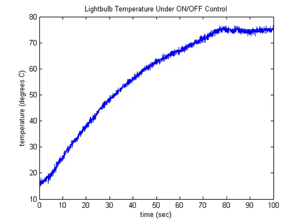
The achieved control outcome is remarkably effective, as it effectively maintains the lightbulb’s temperature in proximity to the desired setpoint without requiring extensive expertise for its design and implementation. Nonetheless, a potential drawback of this strategy is its potential to curtail the lightbulb’s lifespan while not being particularly energy-efficient. Similar considerations are pertinent to various applications involving ON/OFF control. Moving forward, let’s explore a couple of strategies to mitigate the observed temperature oscillations in the lightbulb.
With Low-pass Filter
One approach for reducing the chatter is to add a low-pass filter on the temperature measurement. In the model shown below, we employ a simple first-order filter with a time constant equal to 2 seconds. The filter acts on the ΔT signal to account for the fact that a transfer function assumes zero initial conditions
The resultant controlled behavior is depicted below, illustrating the impact of the low-pass filter on smoothing the recorded temperature signal. An effective way to comprehend this is by envisaging the characteristics of a first-order step response, which essentially refines a swiftly changing signal (a step) by rounding off its edges. Notably, a greater time constant accentuates the rounding-off effect, consequently slowing down the filter’s response. Alternatively, one can perceive the filter as executing a moving average of both current and preceding temperature measurements. This perspective can be derived from a discrete-time rendition of the filter’s transfer function. With a lengthier time constant, the moving average accords more significance to past measurements in the computation.
This filtering technique could have been applied during the creation of our black box plant model. However, an inherent limitation of real-time implementation with a low-pass filter is that it introduces a delay to the signal, which is evident in the illustration below.
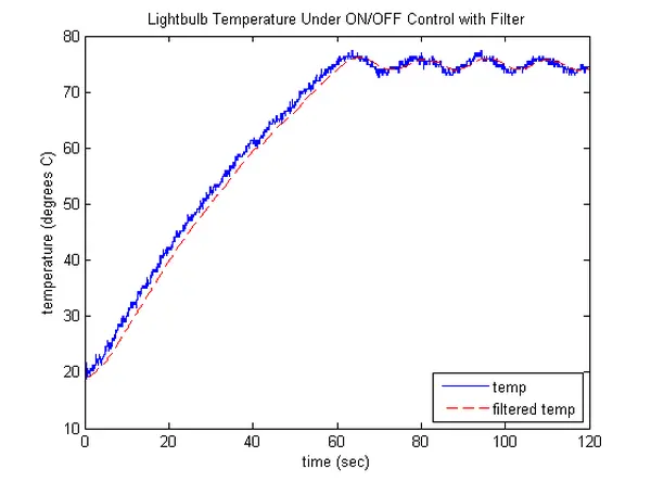
In addition to mitigating noise in the temperature measurement signal, the filter also decreased the frequency at which the lightbulb was cycled on and off, potentially enhancing the lightbulb’s lifespan and efficiency. However, a trade-off exists, as the controlled temperature might deviate further from the desired temperature. The balance of these effects can be influenced by altering the filter’s time constant. This influence stems from viewing the low-pass filter as a moving average. In the absence of a filter, the lightbulb promptly switches off when the temperature surpasses the desired level, and vice versa. With a moving average, the lightbulb doesn’t promptly switch off upon reaching the threshold, as the average is still influenced by prior, lower measurements. It necessitates a series of recent measurements above the threshold to offset the impact of the older, sub-threshold measurements.
With Dead band
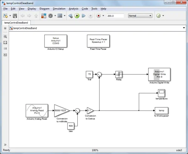
An alternative strategy for mitigating the frequent on-off cycles of the light bulb involves using a dead band. This concept is demonstrated in the model depicted below, utilizing a Relay block. The Relay block functions akin to a switch with hysteresis, meaning it employs distinct criteria for transitioning between “ON” and “OFF” states. In this instance, the dead band is configured at +2/-2 degrees. To clarify, when the measured temperature exceeds the desired level by 2 degrees (77 degrees in this scenario), the lightbulb switches off. Conversely, it switches on when the temperature dips 2 degrees below the desired level (73 degrees in this instance).
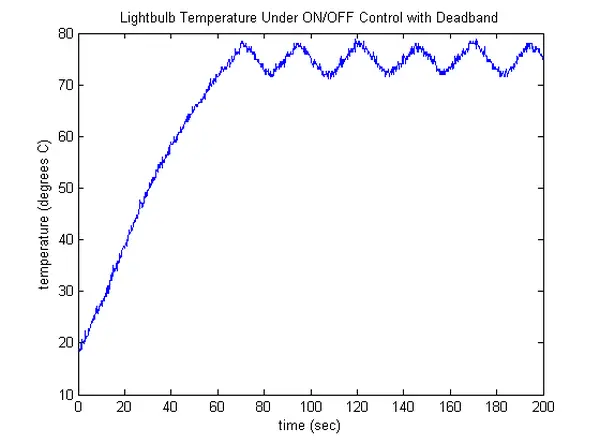
The resultant regulated temperature is illustrated below, displaying a behavior akin to that achieved through filtering. The frequency at which the light bulb undergoes on-off cycles (and the resultant closeness to the desired temperature) can be influenced by adjusting the magnitude of the dead band.
P and PI Control
In our previous attempts at temperature control, we utilized ON/OFF control, where the lightbulb was either fully on when the error was positive or completely off when the error was negative. A more advanced approach to control would involve modulating the lightbulb’s intensity proportionally to the extent of temperature error (and eventually, in proportion to the integral of the error as well). In simpler terms, if the lightbulb was significantly too cold (large error), it would be illuminated brightly; however, if the lightbulb was only slightly below the desired temperature (small error), it would be illuminated dimly. This strategy, where the control effort corresponds to the error’s proportion, is known as Proportional Control or P Control. In mathematical terms, it is expressed as control = KP. error. While this control approach might not yield improved performance compared to the ON/OFF methods used so far, considering the system’s relatively slow and comprehensible dynamics, this exercise will enhance our understanding of P and PI control and how they apply in various scenarios.
P Control
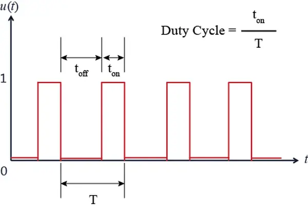
Within our system, we manage the lightbulb’s temperature by cyclically linking and disconnecting it from the AC power source. In this manner, we lack the capability to modulate the lightbulb’s brightness—it’s either connected to the power or it’s not. Nevertheless, we can approximate a continuous P control strategy through the utilization of Pulse-Width Modulation (PWM). In the realm of Pulse-Width Modulation, the input signal takes the form of a pulse train, specifically a square wave, maintaining a constant period (frequency) as it toggles between 1 and 0 (fully on and fully off, respectively, as we’ve demonstrated). The degree of “intensity” in the control is influenced by altering the proportion of time during which the input remains in the “on” state. This proportion is referred to as the Duty Cycle. The depiction of a PWM signal is provided below.
When considering a first-order system, as we’ve encountered here, it’s conceivable to envision the potential behavior of the lightbulb’s temperature if the PWM signal’s period were exceedingly prolonged. This scenario would yield a first-order step response ascending toward a stable value (when active), succeeded by the temperature subsiding to the ambient level (when inactive). However, in practical terms, the PWM signal’s period is intentionally kept short (frequency elevated) in comparison to the dynamics of the controlled system. This design ensures minimal time for the output to either rise or decline significantly. Consequently, by varying the duty cycle of a PWM input, an effect of an almost seamless transition in the output can be achieved.
The provided model below showcases the application of a P Control strategy to our lightbulb system. The implementation of the PWM signal is carried out through the displayed Analog Write block. This block represents the duty cycle as an 8-bit value (2^8 = 256). Hence, the input to the Analog Write block must fall within the range of 0 to 255. In this range, 0 signifies a 0% duty cycle, while 255 corresponds to a 100% duty cycle. The saturation block is incorporated to ensure compliance with these limits. The resulting PWM signal is produced on Digital Pin 9, the same pin we have been utilizing. It’s important to note that digital pins capable of generating a PWM output are identified on the Arduino board by the presence of the ~ symbol.
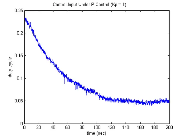
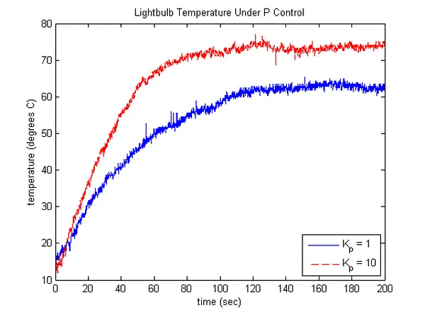
We will initiate by selecting a proportional gain of Kp = 1 without any specific rationale. The resultant temperature profile using this gain is depicted below. Notably, the resulting profile exhibits a notable degree of steady-state error in comparison to the provided reference temperature of 75 degrees Celsius.
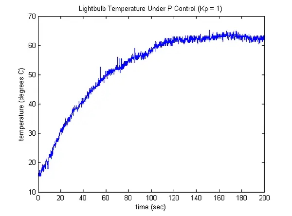
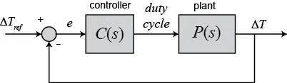
This outcome is in line with our expectations, given the earlier derived plant model, P(s) = 83.5/(66s + 1), which indicates that the resulting control system is of type 0. To gain deeper insights into the observed behavior and the impact of the proportional gain in a broader sense, let’s conduct some analysis. An idealized depiction of our control system is illustrated below. It’s worth noting that the feedback loop is expressed in terms of ΔT, as opposed to T, in order to maintain linearity in our plant with zero initial conditions.
For this particular system with C(s) = Kp and the previously defined P(s), the closed-loop transfer function can be expressed as follows.
![]()
Upon examining the provided information, it’s evident that the closed-loop system possesses a DC gain of G{cl}(0) = 83.5Kp/(1 + 83.5Kp). Even when setting Kp = 1, the DC gain remains very close to 1, implying that the steady-state output of the control system should be closer to the 75-degree reference than it currently is. While it’s reasonable to consider the influence of environmental conditions or changes in the bulb itself, these factors alone can’t fully account for the magnitude of the observed error. The discrepancy between prediction and observation arises from the fact that our model was developed for a step input of 1, representing a 100% duty cycle. Upon analyzing the control input generated for Kp = 1, it becomes apparent that the lightbulb operates with a duty cycle significantly below 100%.
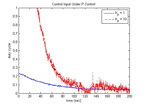
Upon reviewing the derived expression for the DC gain, it becomes evident that elevating Kp will progressively bring the steady-state gain closer to 1. An equally noteworthy observation is that an augmented Kp value will result in an increased commanded duty cycle, thereby approaching the conditions under which our plant model, P(s), was originally developed. A more detailed examination of the closed-loop transfer function reveals that it maintains a first-order nature with a pole located at (1+83.5K_p)/66. Consequently, as Kp is increased, the system still exhibits a first-order type response, but with a quicker convergence to steady-state. Elevating Kp yields the following temperature profile and necessitates the subsequent control effort.
Another option, instead of raising Kp, is to adjust the reference T{ref} in a way that aligns the steady-state temperature with the desired value. Nevertheless, this approach necessitates a dependable and consistent model to accurately determine the scaling factor. Another avenue to explore is introducing integral action into the controller. This will be our next endeavor.
PI Control
Incorporating a component in our controller that is proportional to the integral of the error results in what is known as a Proportional-Integral Controller or a PI Controller for brevity. In mathematical terms, this controller is represented as C(s) = Kp + Ki/s. The inclusion of such a controller renders the feedback control system as type 1, implying that it should nullify the steady-state error to a constant reference (essentially a step response). Analyzing the revised closed-loop transfer function displayed below allows us to delve deeper into this concept.
![]()
For this revised closed-loop transfer function, the DC gain equates to 1. Thus, we can confirm that zero steady-state error will be achieved for a constant reference. As the value of Ki increases, the rate at which the steady-state error diminishes will accelerate. This phenomenon aligns logically when reflecting on the system’s behavior observed with Kp = 1. Under that P controller, the lightbulb’s temperature settled at a steady-state value below the desired level. Fundamentally, the control effort (duty cycle) reached during steady-state provided energy to the bulb at a rate that precisely balanced the rate at which heat was being dissipated to the surroundings. The control input remained unchanged due to the temperature error plateauing and the control effort maintaining proportionality to the error. However, with integral control, the control effort will persistently increase until it eradicates the steady-state error. Integration effectively accumulates the area beneath the error-time graph, resulting in the integral term of the controller augmenting the control effort as it accumulates this error (through area summation).
Incorporating integral control also introduces an additional outcome: our closed-loop system transforms into a second-order response, which might lead to oscillations or overshoot. This consequence is somewhat intuitive. To better understand the implications, we will implement a PI controller with Kp = 1 and Ki = 0.02 and evaluate its response.
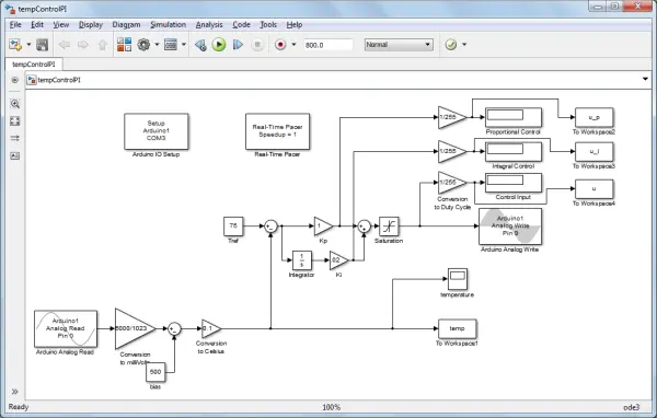
While running this model, pay close attention to the control effort values stemming from both the proportional and integral components of the controller, as displayed. The ensuing temperature profile and control effort for this model are provided below. Initially, the error is substantial and gradually diminishes as the lightbulb’s temperature rises. Consequently, the proportional control effort commences as substantial and subsequently dwindles as the error reduces. However, the integral aspect of the control effort keeps escalating, even as the error magnitude decreases, due to its cumulative nature—this integral continually sums the area underneath the error “curve.” Upon the lightbulb’s temperature aligning with the desired level, the error reaches zero, leading the proportional control effort to also hit zero. Notably, the integral control effort remains considerable, having accumulated all positive error since the inception of the control system. This occurrence is termed “integrator wind-up.” Consequently, the lightbulb persists in heating up for a period, overshooting its intended temperature due to the influence of the integrator. At this juncture, the error turns negative, and the proportional control effort becomes negative as well. Although the integral control effort remains positive, it gradually diminishes. This process of unwinding the integrator unfolds over time. Furthermore, the temperature may subsequently fall below the desired level as it decreases. This illustration exemplifies why our closed-loop system has evolved into a second-order system, indicating it can now possess complex poles and potentially oscillate.
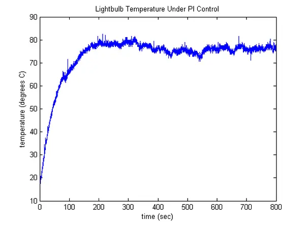
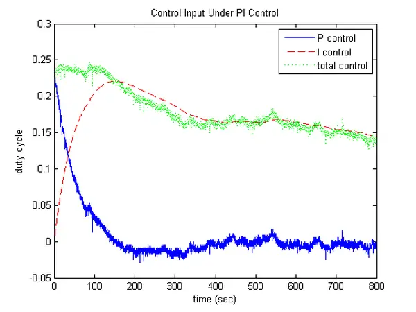
This illustration also demonstrates a prevalent trade-off when incorporating integral control. While its inclusion can assist in reducing steady-state error, it might render the response more oscillatory and sluggish in settling. Tweaking the control gain Ki will influence the balance between these two outcomes. Revisiting our closed-loop transfer function for this feedback system, if we align the denominator with the structure of a standard second-order system, S^2 + 2ζΩns + Ωn^2, we can discern that 83.5Ki = Ωn^2 and 1 + 83.5Kp = 2ζΩn. Consequently, for a fixed Kp, augmenting Ki results in a higher Ωn and a diminished ζ, while sigma = ζΩn remains constant. This showcases how elevating Ki can accelerate the reduction of error (by lowering the rise time due to the larger Ωn), yet this comes at the expense of heightened oscillation (leading to increased overshoot due to the smaller ζ).